In an earlier tutorial we learned the basic of how Vector layers are configured and displayed. This tutorial will expand on that knowledge and teach you how to manipulate layers data.

Vector layers display its geometrical data as points, lines, or polygons using the X and Y coordinates of the features.

• Point: The basic geometrical object, the point, is easiest to represent since the point has no spatial extent and
  can be represented by a single pair of co-ordinates.

• (Poly) Line: A linear object is more complicated since it has a one-dimensional extension and consequently must be represented with a series of co-ordinate pairs describing this extension. In the simplest case of a straight line between two points, the vector model stores the start point and the end point of the line. More complex lines need several pairs of coordinates, one at each breakpoint, where the line changes direction. Smooth real world objects, like for example rivers that change direction more or less constantly, will have to have an indefinitely large number of breakpoints (pairs of co-ordinates) in order to be represented correctly.
  • In GIS terminology, the start point and end point of a line are called “node” and the breakpoints in between are called
    “vertex” (vertices in plural).

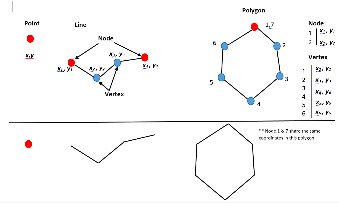
• Polygon: Storing of polygon features is similar to line storing. The polygon is defined by its border line, which in turn is described by start node, stop node and a number of vertices. The only difference is that the coordinates for the start and stop nodes must be the same, otherwise the polygon will not be closed.
  • Centroids serve an important topological function in GIS. In QGIS a single vector area is defined by both (1) a closed boundary (polygon) and (2) an associated centroid. A closed boundary by itself does not define an area. To understand this concept imagine a vector representation of a tray of six doughnuts. As the following figure shows the vector layer would consist of twelve closed boundaries (polygons) but there would only be six “doughnut areas”. Using centroids we are able to indicate which enclosed spaces actually represent doughnut areas and which enclosed spaces don’t represent anything at all. Space that doesn’t represent anything is referred to as “null space”. In the case of the doughnut map, any space that isn’t occupied by doughnut is considered null space. The category number is a code for what the area represents. In the case of the landice layer the centroid becomes more evident when digitizing or labeling, we will see this later in this and other tutorials. In the doughnut map a category value of 1 indicates that the area is occupied by doughnut.

• The GIS software can thus distinguish between the three geometric objects simply by looking on the list of co-ordinate pairs used to describe it. If it is a point, there is only one pair of co-ordinates, if the object is composed of several pairs of co-ordinates it must be a line and if the co-ordinates for the start node and stop node are the same, the object is a polygon.

Activity 1: Change Display Properties of Vector Layers

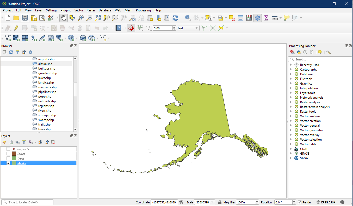
Open a new project and load and display the following layers. Place the layers in the order shown below (points on top) for best viewing.

• airports
• lakes
• trees
• alaska

Centroids

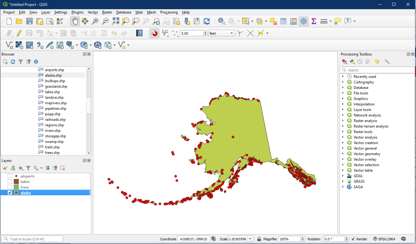
To visualise centroids that were mentioned earlier, do the following. First turn off all the layers except for alaska. Have a look at what the alaska layer looks like – it is composed of many polygons.

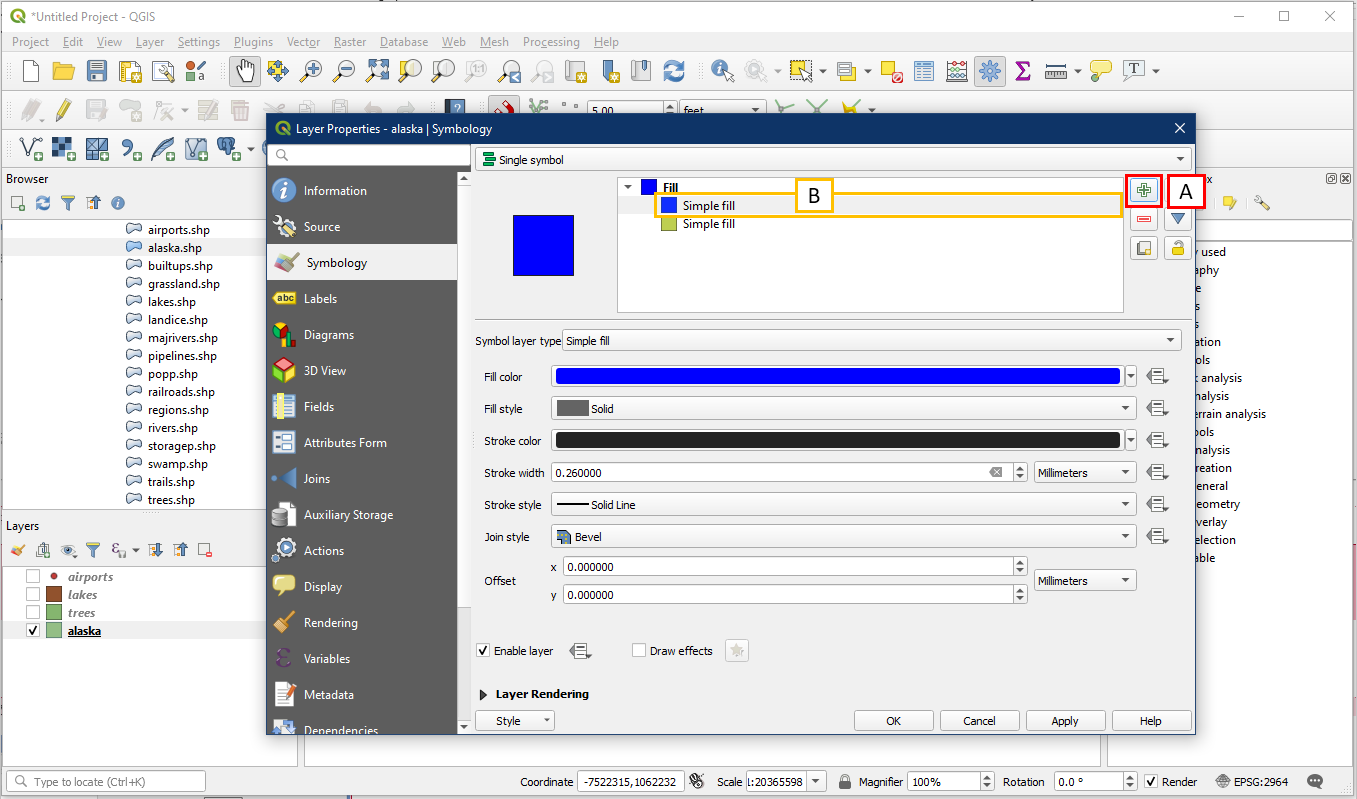
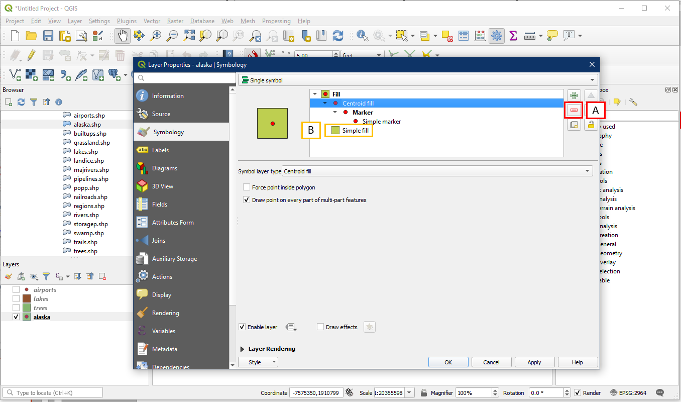
Right click on the alaska layer in the Layers panel and choose Properties > Symbology. By default, under Fill it should contain a Simple fill. Now click the “+” button (A), which should add a second Simple fill on top of the original Simple fill (B).

Select this layer and change from Simple fill to Centroid fill, and OK.

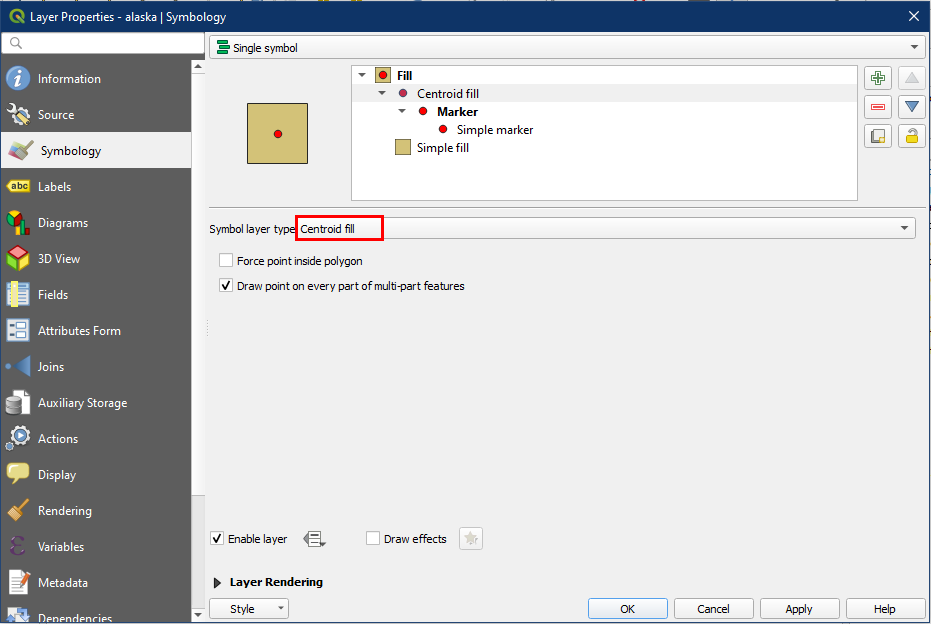
In the Map View you will see dots on top of the original layer symbol, representing a centroid in the middle of each polygon. You will note that there are many more centroids along the coast, this is because the coast is made of numerous tiny small polygons (islands). Zoom in for a better view if you wish.

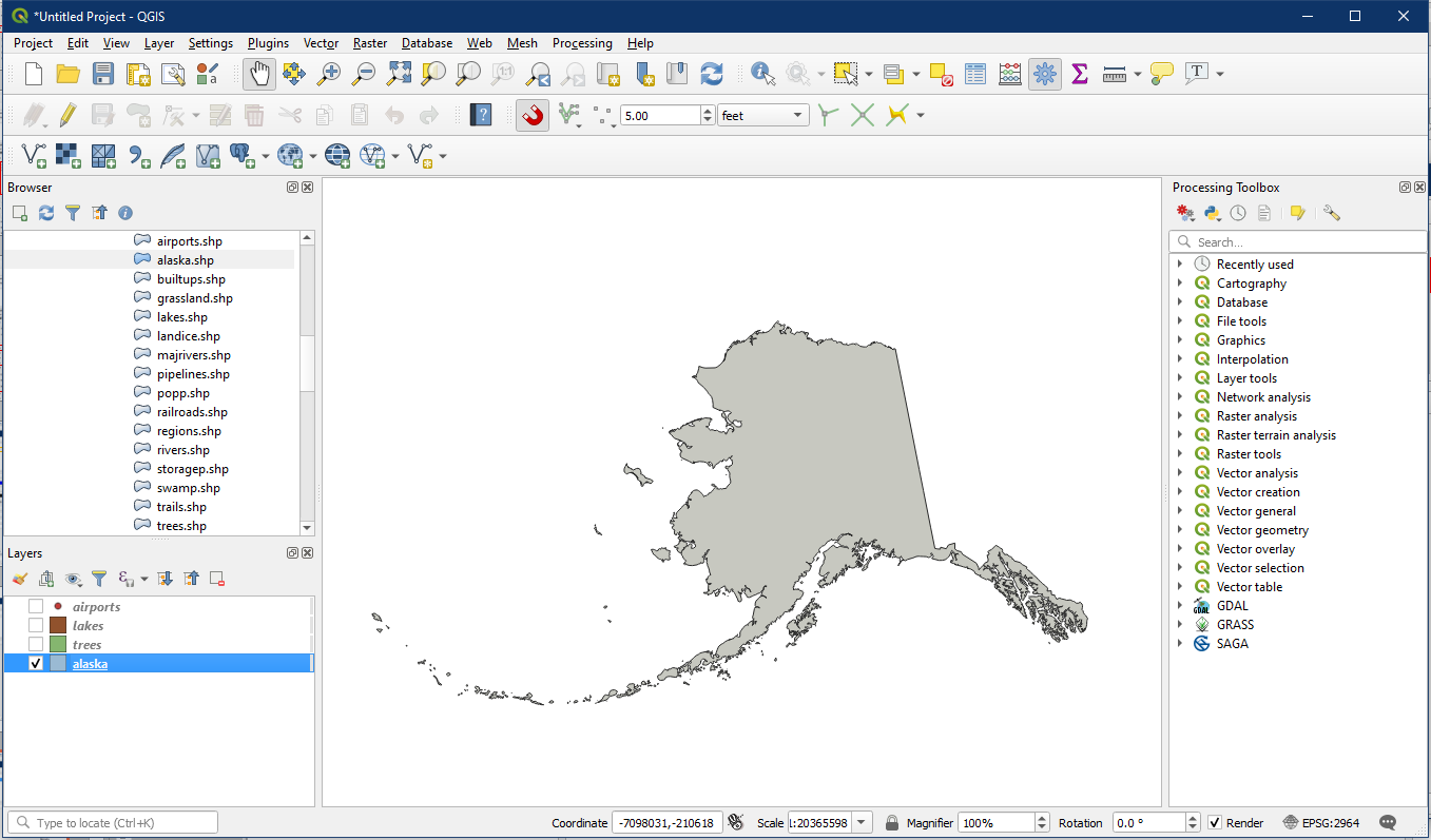
Go back to the alaska layer properties, select the Centroid fill and click the “–“ button (A) to remove this layer so that only the original Simple fill remains in the symbology. Select the original Simple fill (B) and change the fill colour to a light grey (refer to Tutorial 4).

Symbols

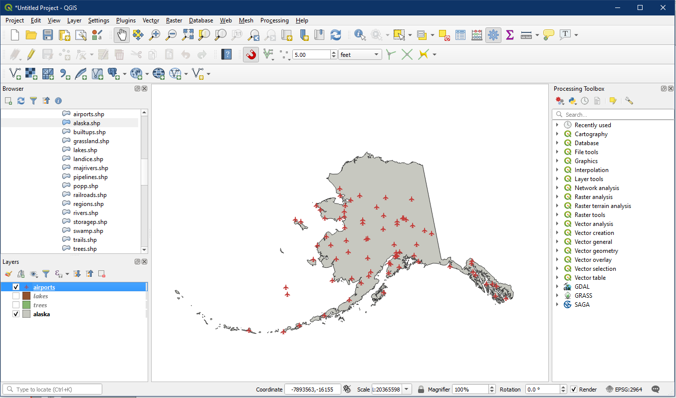
Turn on the airports layer. Right click on the airports layer > Properties > Symbology. Under Marker, the default symbol layer type should be Simple marker.

In Simple layer type change from Simple marker to SVG marker. In the bottom panel you will see SVG Groups and can select the transport category. Look at the choices of symbol groups, these may serve you well in upcoming labs or assignments. In the image below choose an airplane and adjust the Fill colour and Height/Width.

It should look similar to this.

Colour Classifications

Some vector layers contain different classifications for various attributes. Using labels is not always suitable. In this example we are going to learn how to colour classify vector layers based upon an attribute.

Turn off the airports layer and turn on the trees layer. Right click on the trees layer and select Open Attribute Table. A table for the trees layer will pop up and we will see the VEGDESC field. This describes the different types of trees in Alaska.

Now open Properties and in the Labels section choose Single labels. The label Value should be VEGDESC. Click OK.

You will notice the confusing array of labels which is less than ideal for the map reader.

Rather than use labels ineffectively it may be better to illustrate the different tree classifications based upon colours. So go back to the trees layer properties to turn off labelling, by going under labels and change Single labels back to No labels.

In the trees layer properties go to the Symbology tab. Then do the following:

1. The default symbol should say Single symbol. Click on the dropdown and change it to Categorized
2. Under Value choose the field VEGDESC
3. Under Colour ramp, ensure that Random colours is picked.
4. Click the Classify button, which will populate the category box (E) to include all the vegetation types available
5. In the box with the list of categories, you can change the individual symbol colour by double clicking the coloured square or by clicking the coloured box beside the Symbol option

In the Layers panel it should now show the different tree categories we classified. Notice that there is one category that’s empty. This empty category is used to colour any objects which do not have a VEGDESC value defined (NULL value). It is important to keep this empty category for data keeping purposes. You may like to change the colour to more obviously represent a blank or NULL value, or alternatively, you can simply turn off the NULL values by unchecking the checkbox in the Layers panel.

 

Activity 2: Creating a New Vector Layer through Selection

In some instances we want to extract a feature(s) from a vector layer and create a new vector layer with only that feature(s). In later tutorials we will learn more advanced methods for this but for now this will prove useful.

Turn off the trees layer and turn on the lakes layer. As an example, we want to find and highlight Iliamna Lake on the map.

Right click on the lakes layer and select Open Attribute Table. Under the NAMES column find Iliamna Lake. One trick is to click the NAMES box (A) which will sort the records. Once you find Iliamna Lake, select the number beside the record (B), and the record will now be highlighted in blue in the attribute table. On the map the lake will be highlighted in yellow (C). Clicking the Deselect All button (D) will unselect any highlighted features in both the table and on the map.

In the attribute table, select Iliamna Lake again. Right click on any part of the blue highlighted record and select Zoom to Feature to zoom to the feature on the map. This is a good method to use if there are many records and you cannot locate the highlighted feature on the map manually.

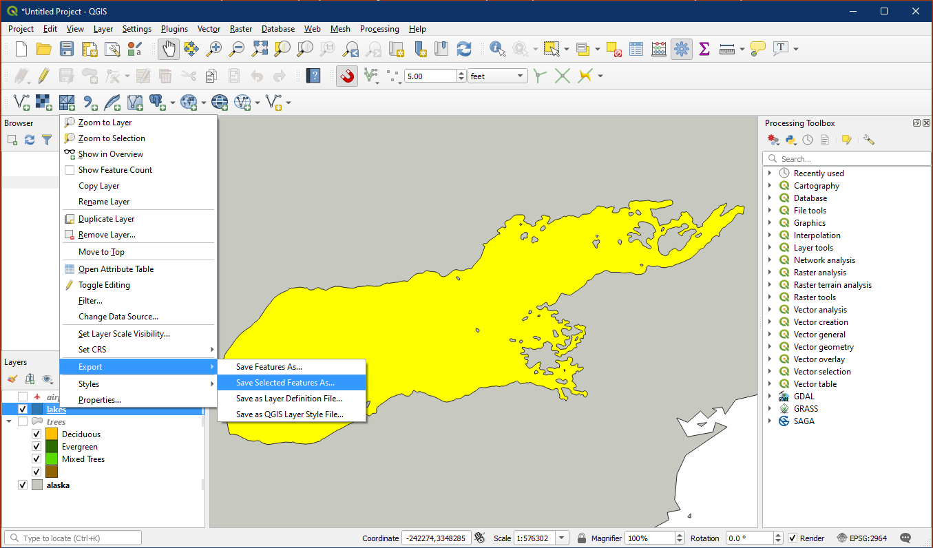
Make sure the Iliamna Lake is still selected. Right click on the lakes layer in the Layers panel > Export> Save Selected Features As.

In the dialog box do the following:

1. For format choose ESRI Shapefile. This is the most common file format for vector data
2. For File name, click the “…” button and a “Save Layer As” window will pop up.
3. In the new window locate the folder where the original lake data is stored. Enter a new file name e.g. Iliamna_Lake, and select ESRI Shapefile (.shp). Press Save. This will populate the File name box beside the “…” button in part B.
4. Ensure that Save only selected features is checked

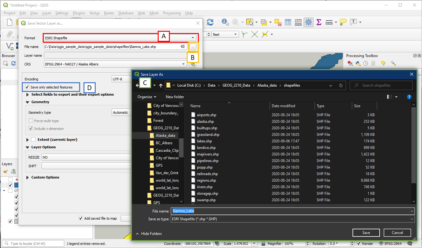
IMPORTANT NOTE: Do not enter your file name directly into the File name box because it will only create a temporary layer that will be lost when you exit QGIS. Always use the “…” button to save your layer instead.

A new layer should now be created showing Iliamna Lake.

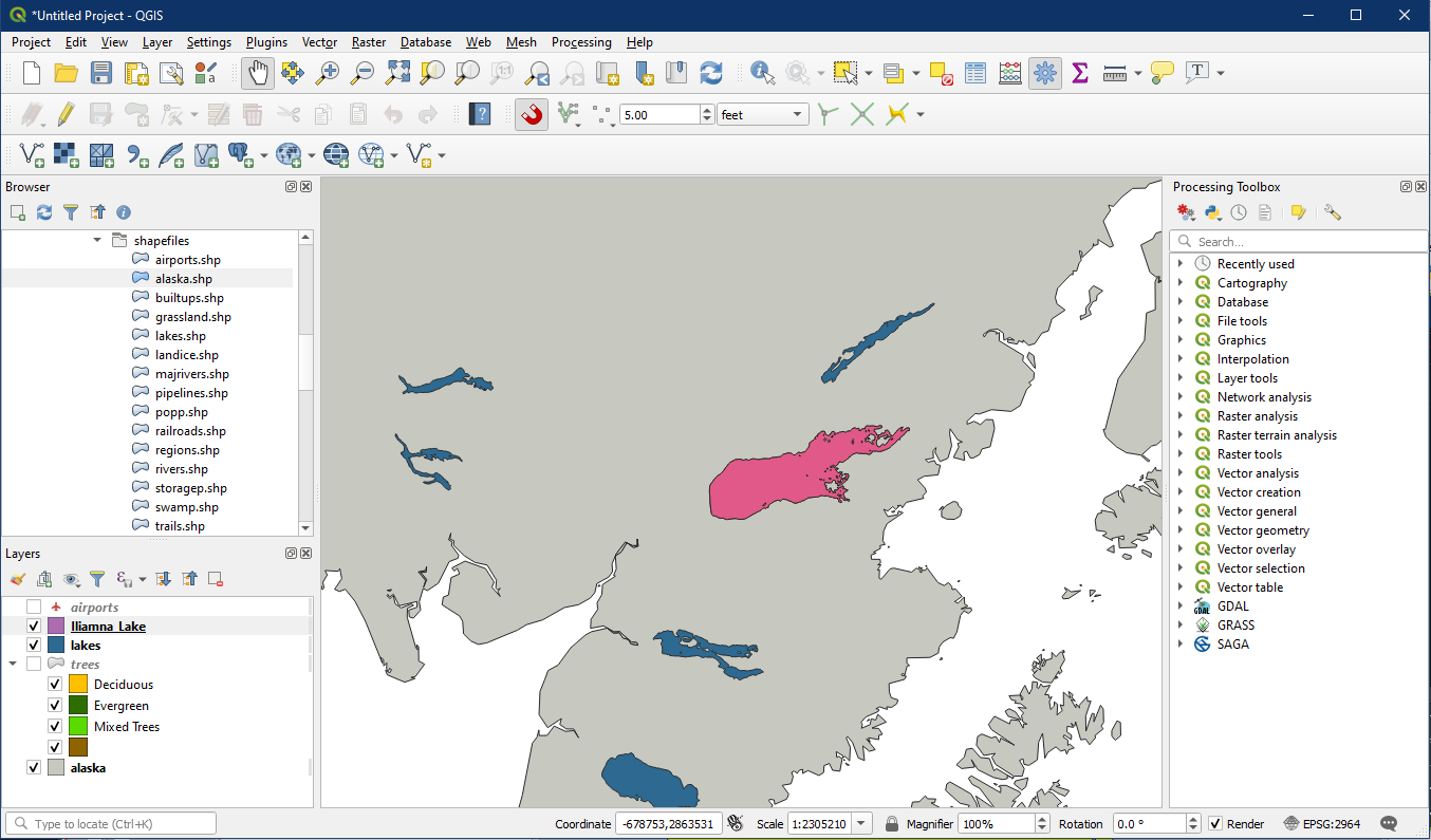
Turn on the other layers. You can also change the Lake Iliamna colour and add a label if you like. Great work! Make sure to save this project e.g. Tutorial_9 so you don’t lose your hard-earned changes.