We have been working with the Alaska database and its spatial components, specifically the vector layers (shapefiles) showing airports, rivers, lakes, etc.

This tutorial introduces the other key component of a GIS database, the attribute data. In Vector-based data structure geographic features or spatial entities are represented points, lines, and polygons (areas) which may contain certain attributes (or information) related to their geographic location. Attributes are stored in databases in tabular form. The ability to visualize, query, manipulate, and analyse data is critical to GIS. For example, the Airports shapefile or vector layer contains 76 rows of data to represent 76 airports in Alaska. The attribute information for the spatial entities are stored in separate databases which are linked to the vector layers.

Tabular information is the basis of geographic features, allowing you to visualize, query, and analyse your data. In the simplest terms, tables are made up of rows and columns, and all rows have the same columns. In QGIS, rows are known as records and columns are fields. Each field can store a specific type of data, such as a number, date, or piece of text.

Feature classes are really just tables with special fields that contain information about the geometry of the features. These include the shape field for point, line, and polygon feature classes and the different fields (columns) for annotation feature classes. Some fields, such as the unique identifier number (ObjectID) and Shape, are automatically added, populated, and maintained by QGIS.

Activity 1: Viewing Attribute Tables and Fields

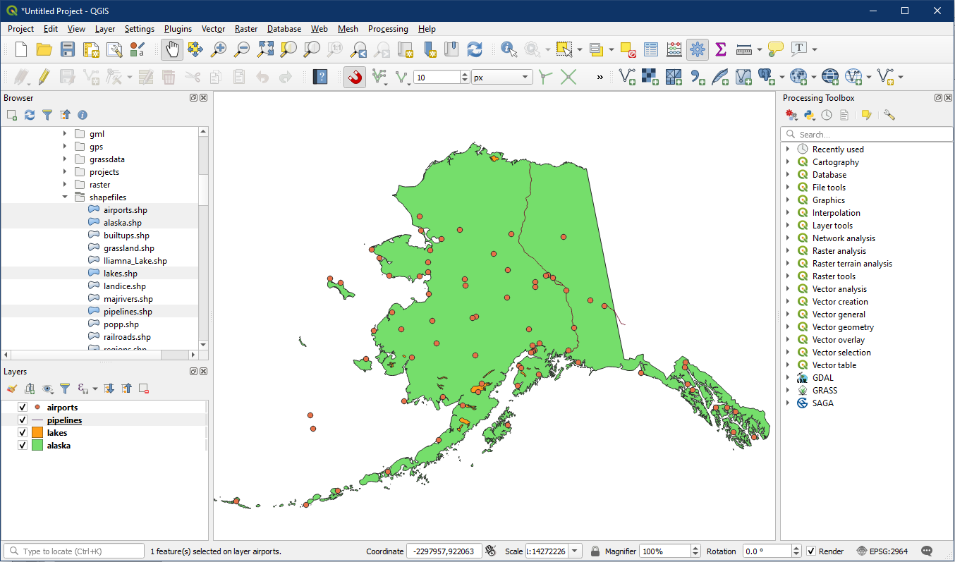
Open a blank QGIS project and using the browser panel locate Alaska_data folder. Locate the following layers and drag them onto the map to add them to the project.

• airports.shp
• alaska.shp
• lakes.shp
• pipelines.shp

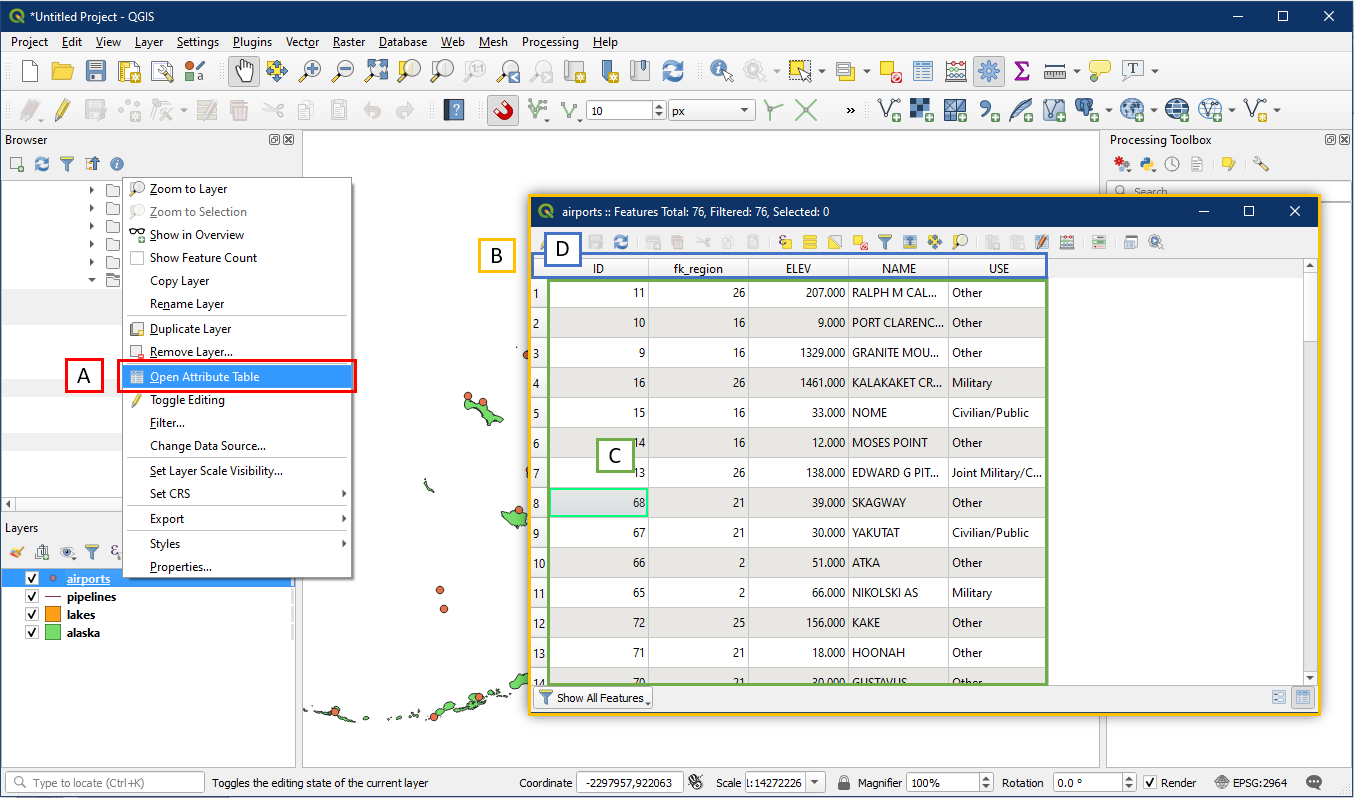
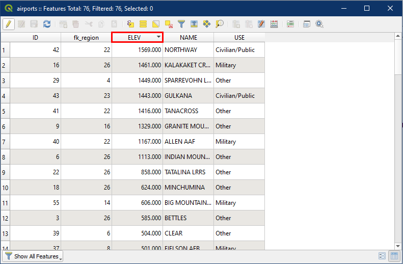
Examine the attribute table for the airports layer by right-clicking the layer and Open Attribute Table (A). A new window (B) containing the attribute table will appear. If you right click on any cell within the table (C) you will see a choice of options for copying the cell, selecting, and locating the feature. Each row in the database is a “record”. The columns are generally referred to as “fields”. The names of the columns/fields are listed across the top of the database table (D).

The scrolling arrows can be used to move through the table to see more columns and records. The column widths can be changed by dragging with the cursor. QGIS attribute database tables are stored in the widely used dBASE (.dbf) format. Field names are limited to 10 characters in the .dbf format. In a .dbf file each field can only contain one “data type” and each record can only contain one data value per field.

To see a list of all fields/columns and data types, right click the airport layer > Properties and look under Fields.

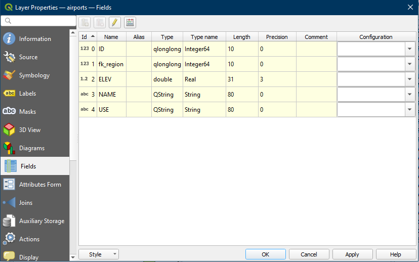
Notice the various Data Types. You will see maximum lengths and precision.

The airports.dbf file has fields with three data types.

• Integer data type fields hold whole numbers (no decimal point). Integers are often used as codes, e.g. 1 means blue, 2 means red etc. Note how in the example the key column, “ID” and “fk_region”, data type is integer.

• Double data type fields that hold “Real” numbers (numbers with decimal points). Note how “ELEV” or elevation is a Real number

• String data type fields that hold strings of alphanumeric characters, e.g. digits, letters and symbols. Note how in the example, the “NAME” and “USE” fields data types are strings.

As has been discussed in class, an important concept is the existence of different “levels of measurement” for attribute data. Generally four levels of measurement are recognized; (1) Nominal, (2) Ordinal, (3) Interval and (4) Ratio. [NOIR]

A question to think about is what data types would be suitable for attributes measured at different levels?  For example, could the character data type be used for attribute measurements made at the interval or ratio level? What data type would be most appropriate for attributes measured at the nominal level? Would it be appropriate for to use the double precision data type for attributes measured at the ordinal level?

In the example the “ID” field is the key. This field ties the attribute database record to the vector layer entity.

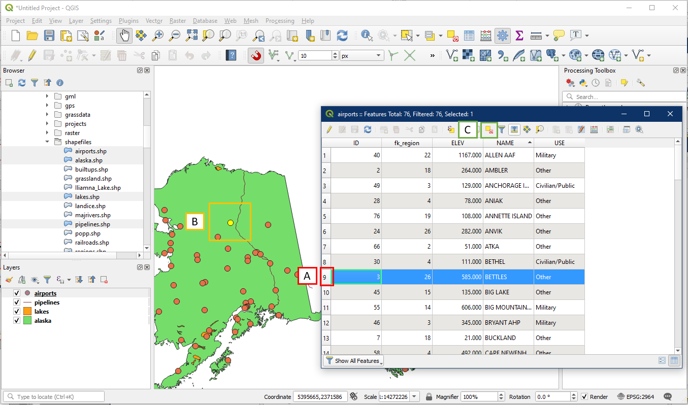
Right click on the airports layer and select Open Attribute Tables. By default, the attribute table is listed in ascending order using the ID field. However we can sort using any field. We can also alternate ascending/descending order by clicking on the field again. For example we can sorted in descending order using the ELEV Field, by clicking on the ELEV field twice (first click to sort by ascending, and second click for descending)

You can select a record from the attribute table by selecting the number associated with it at the very left (A) and the row will be highlighted in blue. This feature will also be highlighted in yellow on the map (B). Press the Deselect All button (C) to remove the selection/highlight.

Activity 2: Adding a New Field in the Attribute Table

Right click on the Lakes layer and select Open Attribute Table. Within the table:

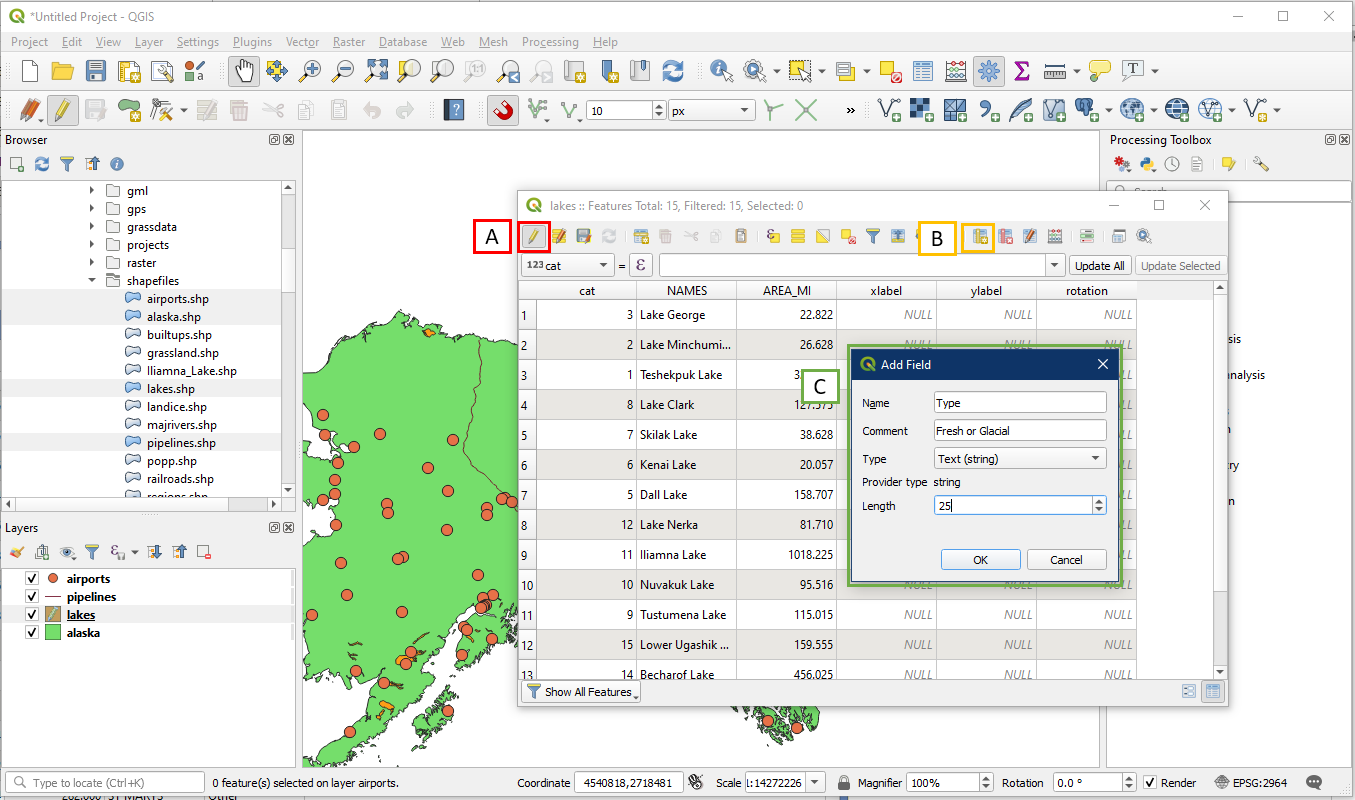
1. Click the Toggle Editing Mode button to turn on editing mode
2. Click the New Field button, which will bring up a new window
3. In the new Add Field window, fill in as shown below (the Comment field is optional). Click OK.

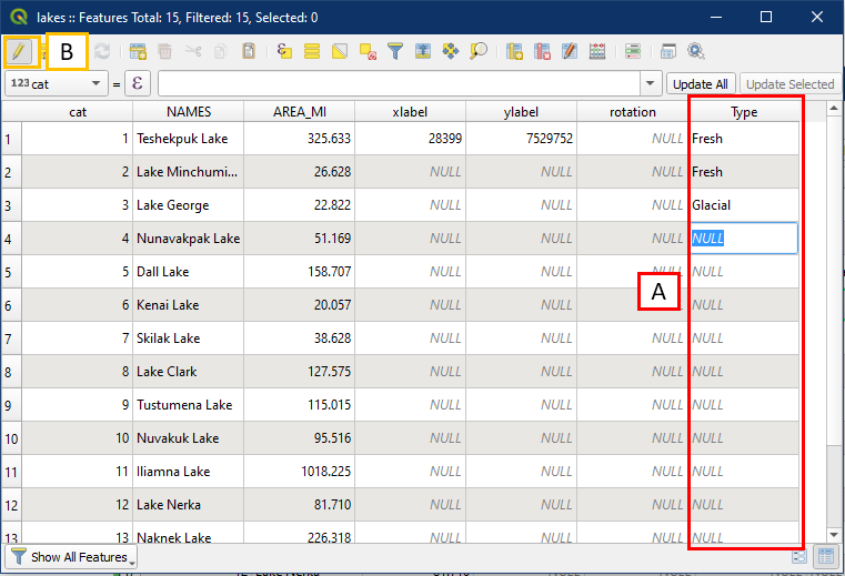
The new field called Type will appear at the end of the row of fields (A). Since editing mode is still on, you can enter values into it e.g. Fresh or Glacial. Now we need to save our changes to the attribute table, so click on the Toggle Editing button (B) again to turn off editing. It will prompt you to save changes to the layer, select Save.

Activity 3: Attribute Table Queries

Attribute table queries are very useful especially when working with large databases containing many records. If you know what you want to search for, it can take significantly less time than manually searching through potentially thousands of records in the attribute table. Right click on the airports layer and select Open Attribute Table. Notice that it has a field for elevation called ELEV as well as a field called USE. We will test out the query tool using these fields.

The first example will involve string (text) data. The USE field is a string data field. For example, we may want to query for all airports used by the military. To do so:

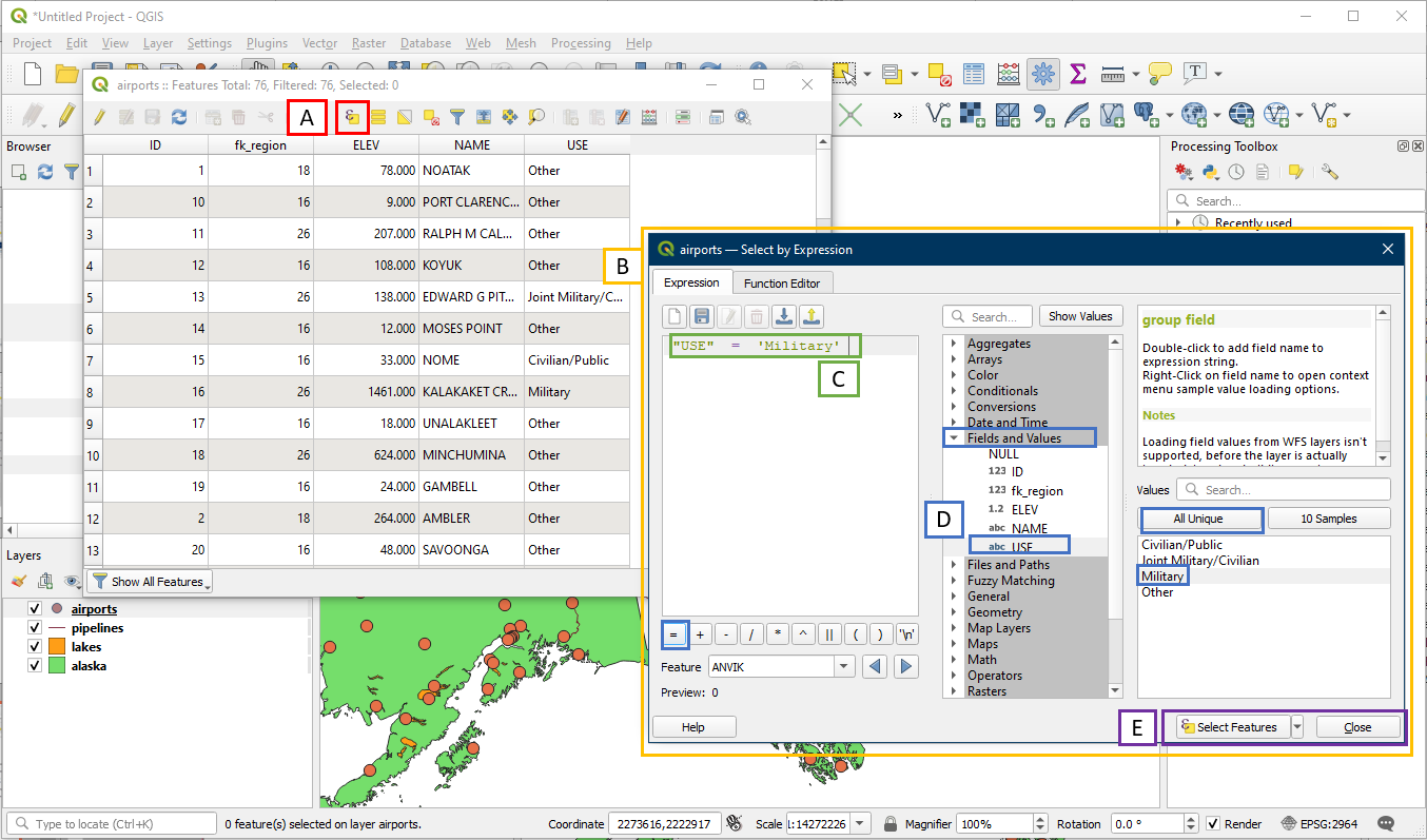
1. In the airport attribute table, click the Select features using an expression button
2. The Select by Expression window will open up
3. In the Expression box, type in“USE” = ‘Military’
4. Alternatively, click the search interface under “Fields and Values” and the “All Unique” button to produce the same outcome
5. Click Select Features, then click Close.

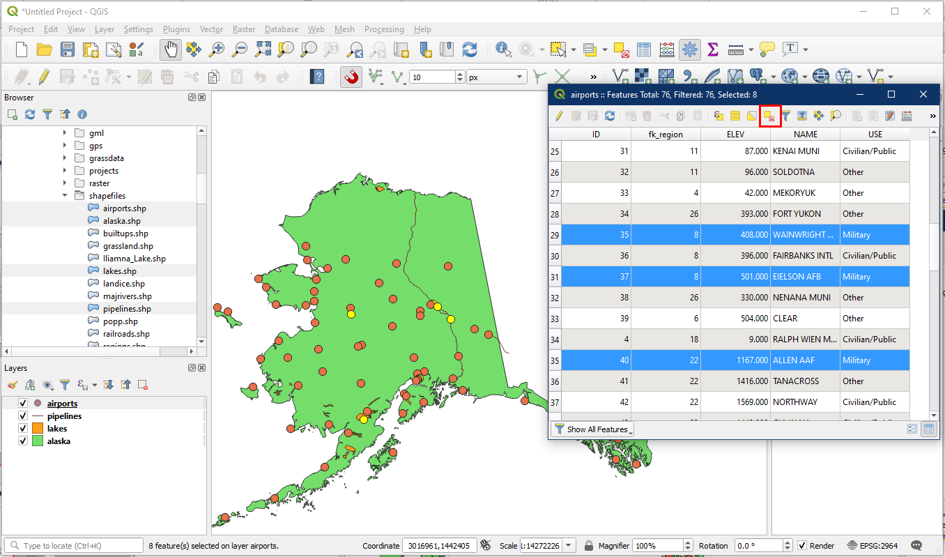
All the airports with a string value of Military within the USE field will now be highlighted on both the attribute table and on the map. Click the Deselect All button to deselect.

We can also query numerical data. This works for both Real and Integer data types.. For example we may want to locate all the airports built near sea level (less than 30m). To do so:

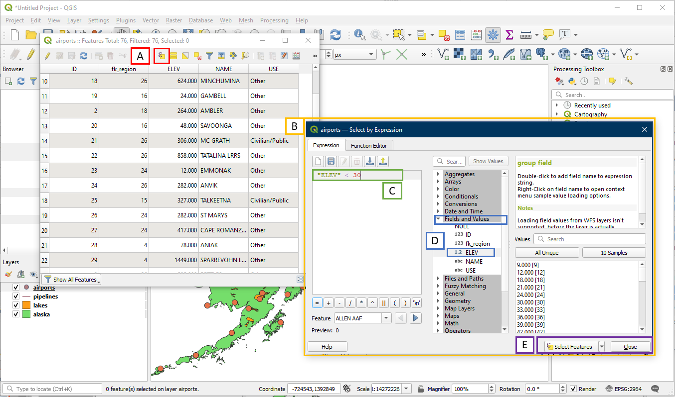
1. In the airport attribute table, click the Select features using an expression button
2. The Select by Expression window will open up
3. In the Expression box, enter  “ELEV” < 30
4. Alternatively, use the interface to select the ELEV field. Since it is a numerical field, the “All Unique” search option does not work well, so you will have to still type in “< 30”
5. Click Select Features, then click Close.

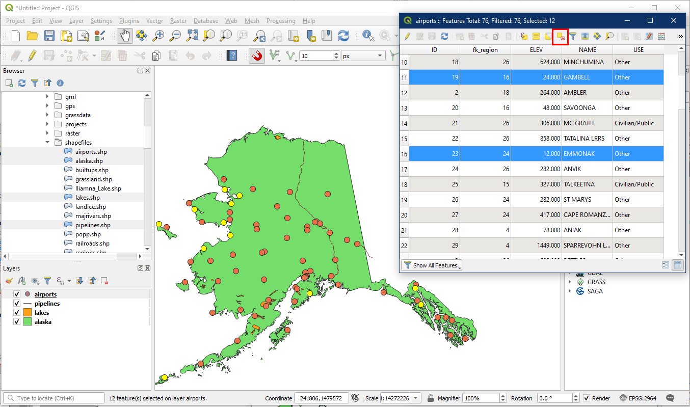
All airports that were listed as having an ELEV value of less than 30 will now be highlighted in the attribute table and on the map. Click the Deselect All button when you are done.

Activity 4: Exporting Attribute Tables

Often as part of a report we may want to have a separate attribute table to accompany the map, so that the attribute data can be easily viewed.

First choose a layer (e.g. airports) to be used to export the attribute table. Right click on it in the Layers panel and select Export > Save Features As.

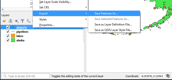
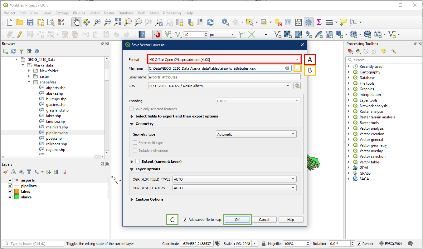
The Save Vector Layer window should open up. Under Format (A), select MS Office Open XML spreadsheet (XLSX). This is the default Microsoft Excel format. Another common spreadsheet format from this list is CSV, which we may use for another time. Under File name, click the “…” button (B) to choose a folder location and file name for the new file. For example within the Alaska data folder create a new folder called tables, and save this file as airports_attributes within. Press OK (C).

Note: Do not directly enter a file name into the blank box for File name, it may not save properly. Always use the “…” button (B).

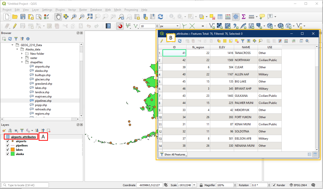
Under the Layers panel, the new attribute file should now appear (A). Notice that it has a “spreadsheet” icon instead of a checkbox and a symbol, this means it is only a spreadsheet table file and cannot be viewed visually. But right clicking on it and clicking View Attribute Table will still bring up the attribute table (B).

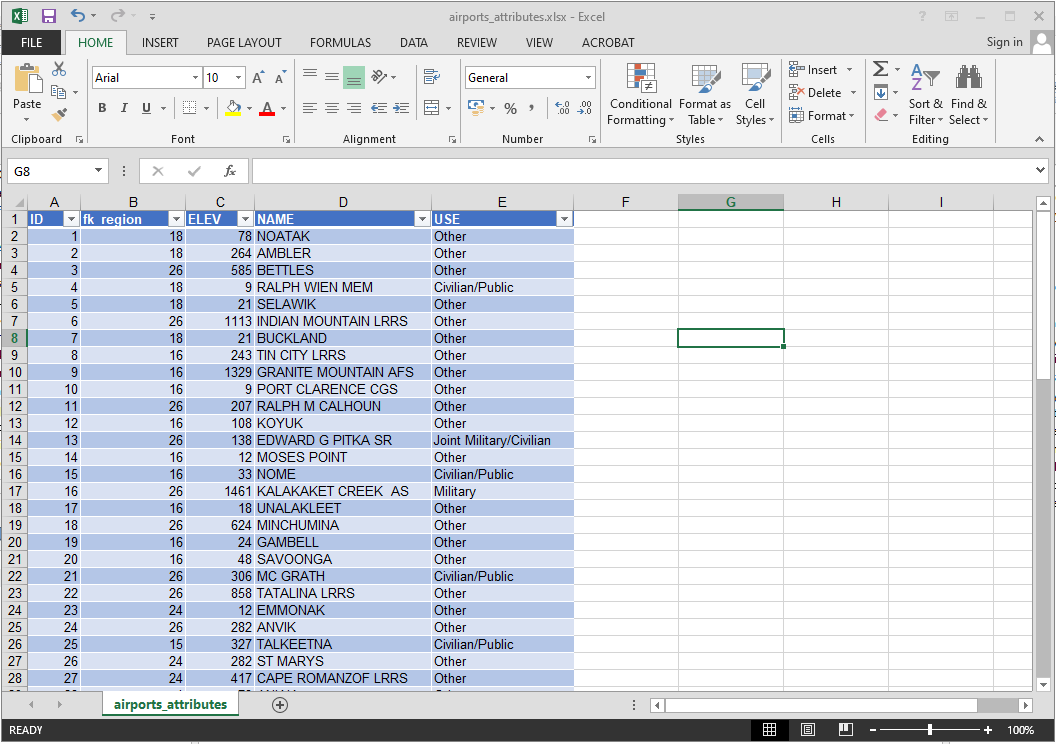
Since this is an XLSX spreadsheet file, we can also open it in Excel instead of QGIS. Navigate to the folder where it is saved and have a look at the table – it will contain the same information as the table within QGIS.

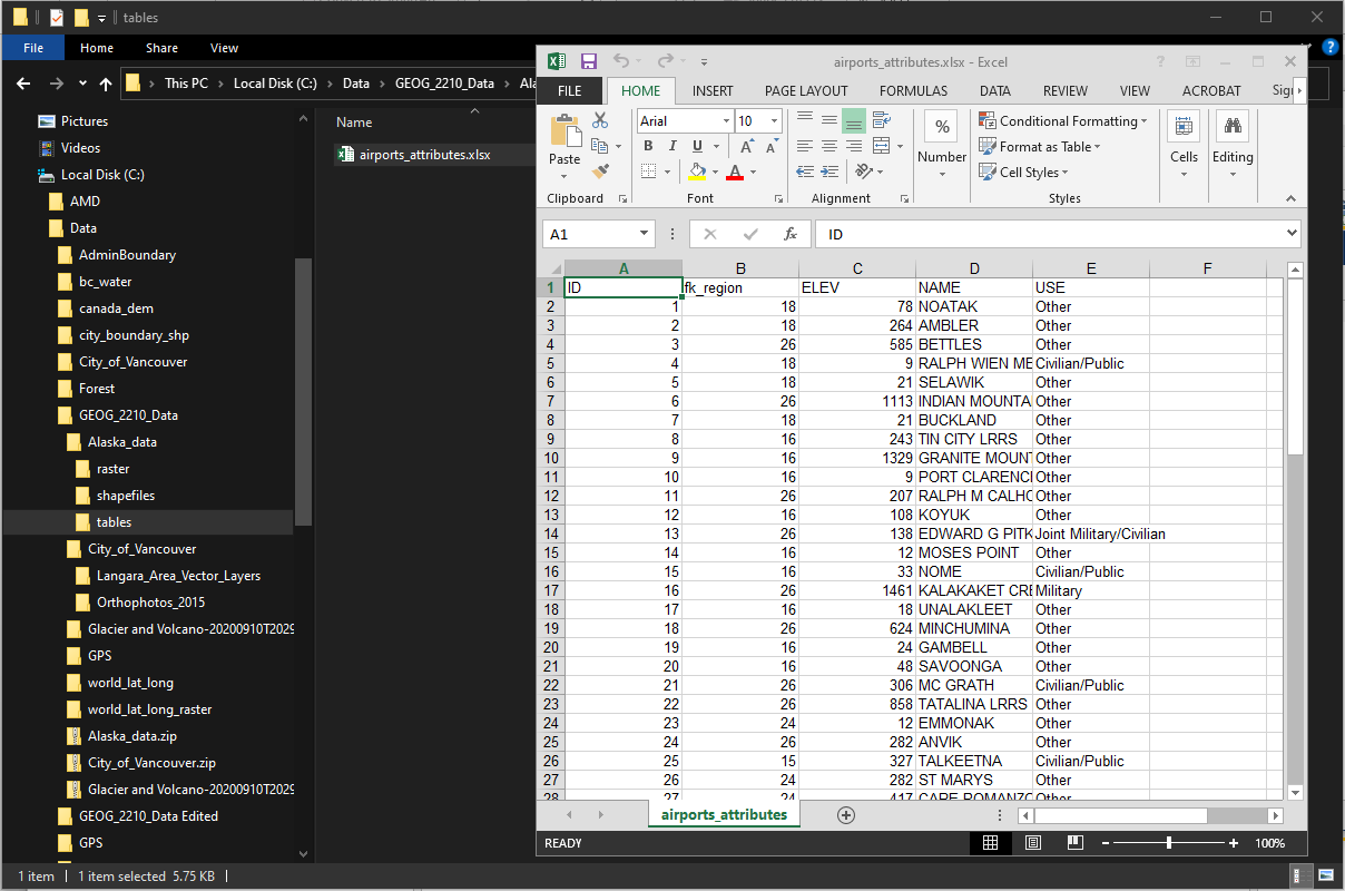
It can also be reformatted in Excel if we want to use it in a presentation or a report.