Opening and displaying Raster layers involves the same processes as the vector layers.

You can add raster layers by using either the Data Source Manager or the Layer Panel. Raster is different from Vector data. Raster data is stored in pixels (cells) with a specific number of rows and columns providing the resolution of the raster data or image.

You can see the resolution of the Raster imagery by adding the raster layer and then right clicking on the layer > Properties.

Information Properties

The Information tab displays basic information about the selected raster, including the layer source path, the display name in the legend (which can be modified), and the number of columns, rows and no-data values of the raster.

Source Properties

Displays the layer’s information, including: the Layer name as displayed in the Layers Panel, the Coordinate Reference System (CRS).

Band Rendering 

A raster dataset contains one or more layers called bands. For example, a color image has three bands(red, green, and blue) while a digital elevation model (DEM) has one band (holding elevation values), and a multi-spectral image may have many bands.

QGIS offers five different Render types. The renderer chosen is dependent on the data type.

1. Multiband color – if the file comes as a multiband with several bands (e.g., used with a satellite image with several bands)
2. Paletted – if a single band file comes with an indexed palette (e.g., used with a digital topographic map)
3. Singleband gray – (one band of) the image will be rendered as gray; QGIS will choose this renderer if the file has neither multibands nor an indexed palette nor a continuous palette (e.g., used with a shaded relief map)
4. Singleband pseudocolor – this renderer is possible for files with a continuous palette, or color map (e.g., used with an elevation map)
5. Hillshade – makes the raster layer appear 3-dimentional by applying shadows based on the elevation values and a theoretical sun elevation/angle

Activity – Displaying Raster Layers

Open QGIS and open your Tutorial_4 project from the previous activity, turn all of your vector layers off.

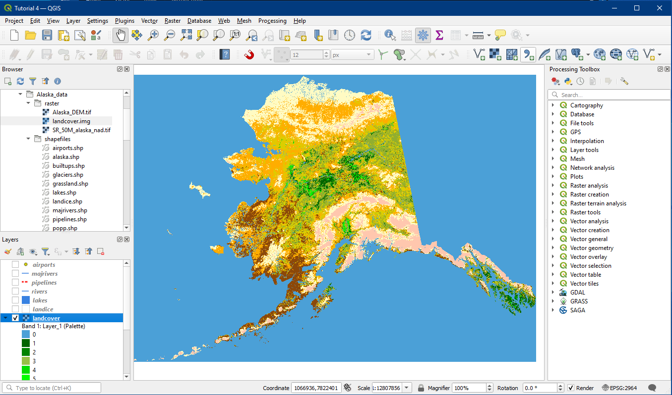
Locate Alaska_data > raster > landcover.img and add this layer to the Layers Panel. Move it to the bottom of the layer list, below the vector layers.The “Select Transformation” window may appear, simply click OK.

Locate Alaska_data > raster > SR_50M_alaska_nad and add this layer to the Layers Panel. Place this layer on top of the landcover raster layer, but below the vector layers.

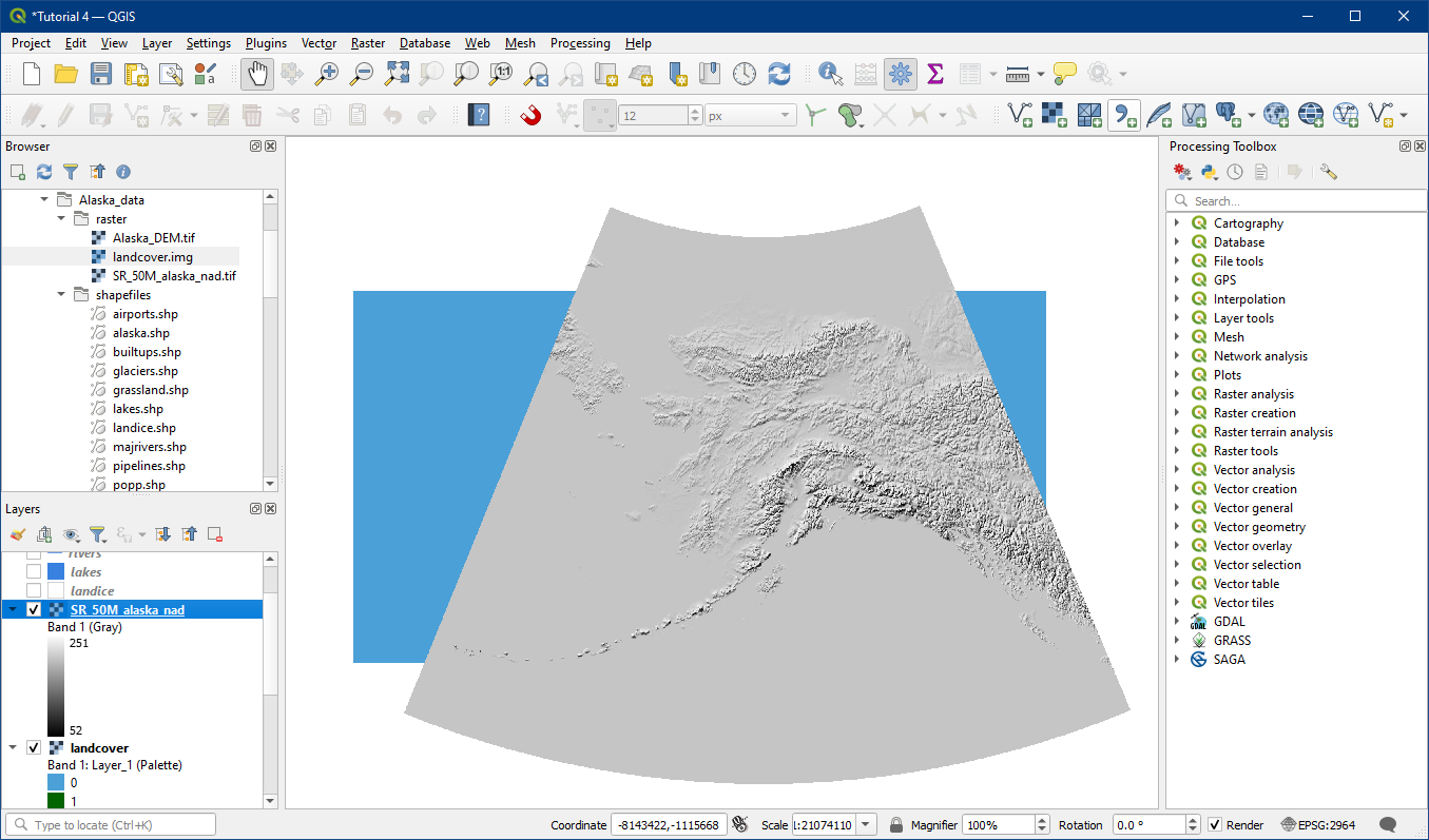
In Layer Properties > Transparency you will see Global Opacity with a slider. Play around with this until you find the best fit for highlighting the topography of Alaska (around 60%).

This is a form of a hillshade or shaded relief layer. You will also notice the different edges on the images and how they do not align this is likely due to their origin from different projections (which we will cover soon). You can also improve the contrast of the shaded relief map by working with blending modes (optional, see Additional Cartographic Tips – Activity: Blending Modes)

You can now turn all of the layers on and view your map of Alaska.

Once you have completed this activity, you can save the Project as “Tutorial_5” in your folder directory.