As we have already learned the spatial-base geometric features are best presented in vector format; whereas the ability to compute statistics on spatial data is best performed using raster formats. This is because most computer languages and mathematical/statistical methods built in to GIS are based upon numbers and binaries. Hence, it is much easier to compute using rasters.

This is not to say that vector lacks some forms of spatial analysis (e.g. TINS, or contour lines for elevation data), but rather that raster is often a preferred method and perhaps a better name would be Raster or Grid analysis.

When wanting to conduct a variety of different forms of analysis it is essential that the two types of data exist in the same format. We will examine the options below.

Activity 1: Raster to Vector

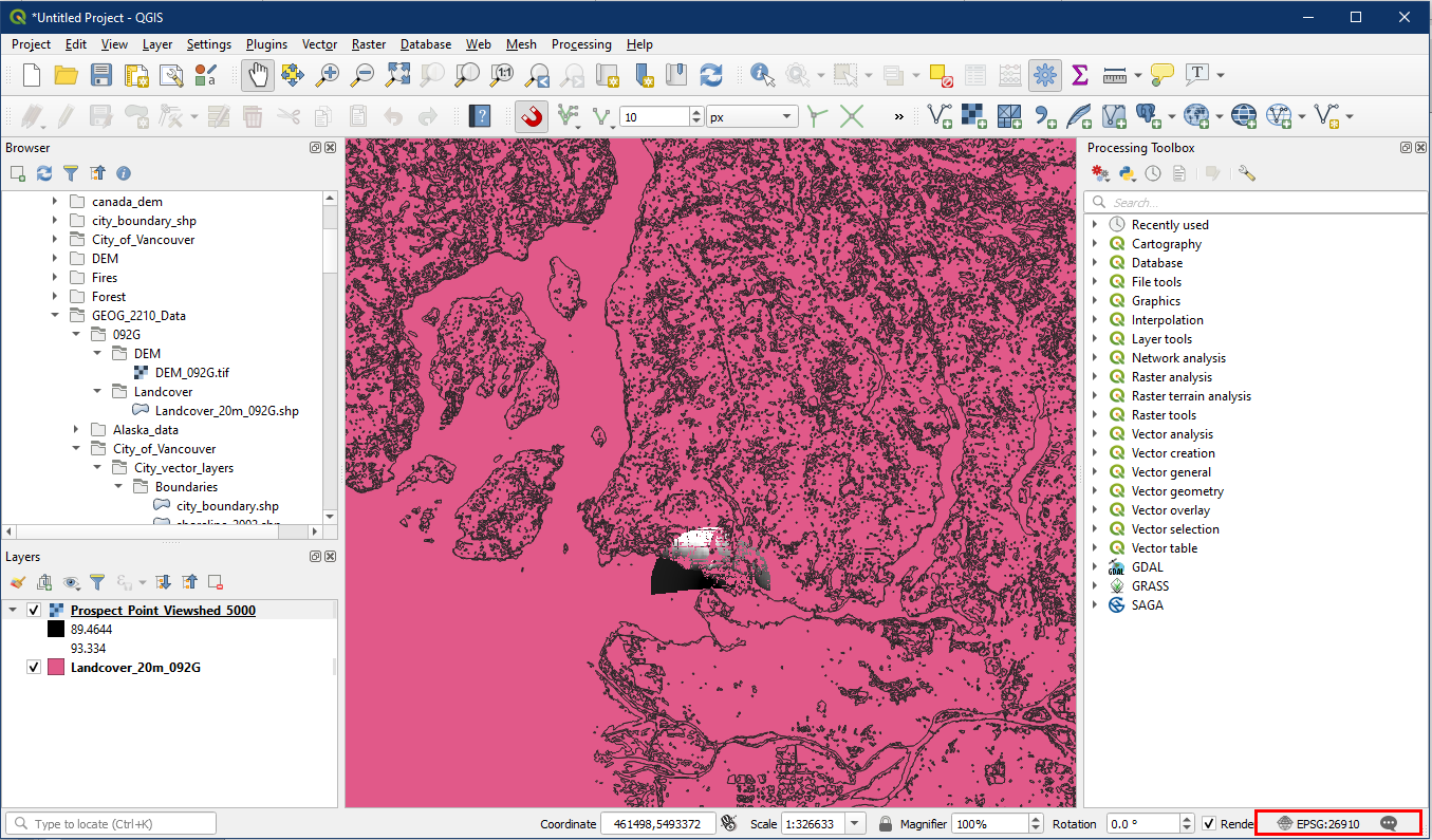
Open a new QGIS project. Add the following layers.

• Landcover_20_092G from the 092G folder
• Prospect Point viewshed layer that we created in tutorial 19

Additionally, ensure the project CRS is in EPSG 26910. The viewshed tool we used in tutorial 19 produces an unknown CRS so want to ensure the project is in the proper CRS.

In order to conduct an overlay analysis we will need to convert the viewshed raster layer into a vector layer. But first we want to produce a reclassified raster layer with a single value instead of a range of different values, this makes the following conversion easier. To do so open the r.reclass tool (recall Tutorial 18) and enter the following settings:

1. For Input raster layer, select your Prospect Point viewshed raster layer
2. In the Reclass rules text enter the following. Note that sometimes you may wish to only keep a smaller subset of this raster (e.g. areas between 45° and 135°) like in the lab assignment
   1. 0 thru 180 = 1
3. Click the “…” button to Save to File, choose a folder and file name for the reclassified viewshed layer

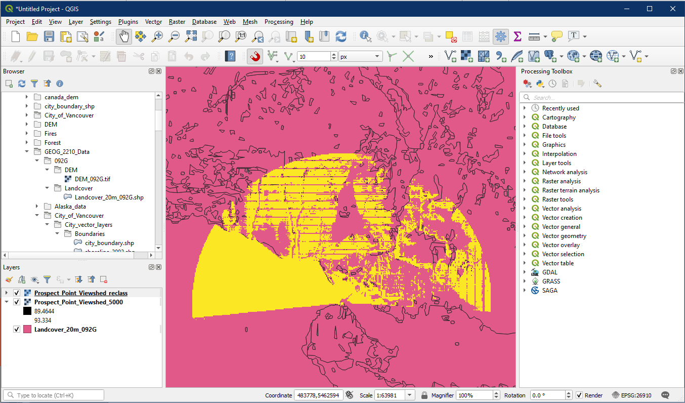
Now our viewshed area contains only one raster value, and it can now be converted to a vector layer.

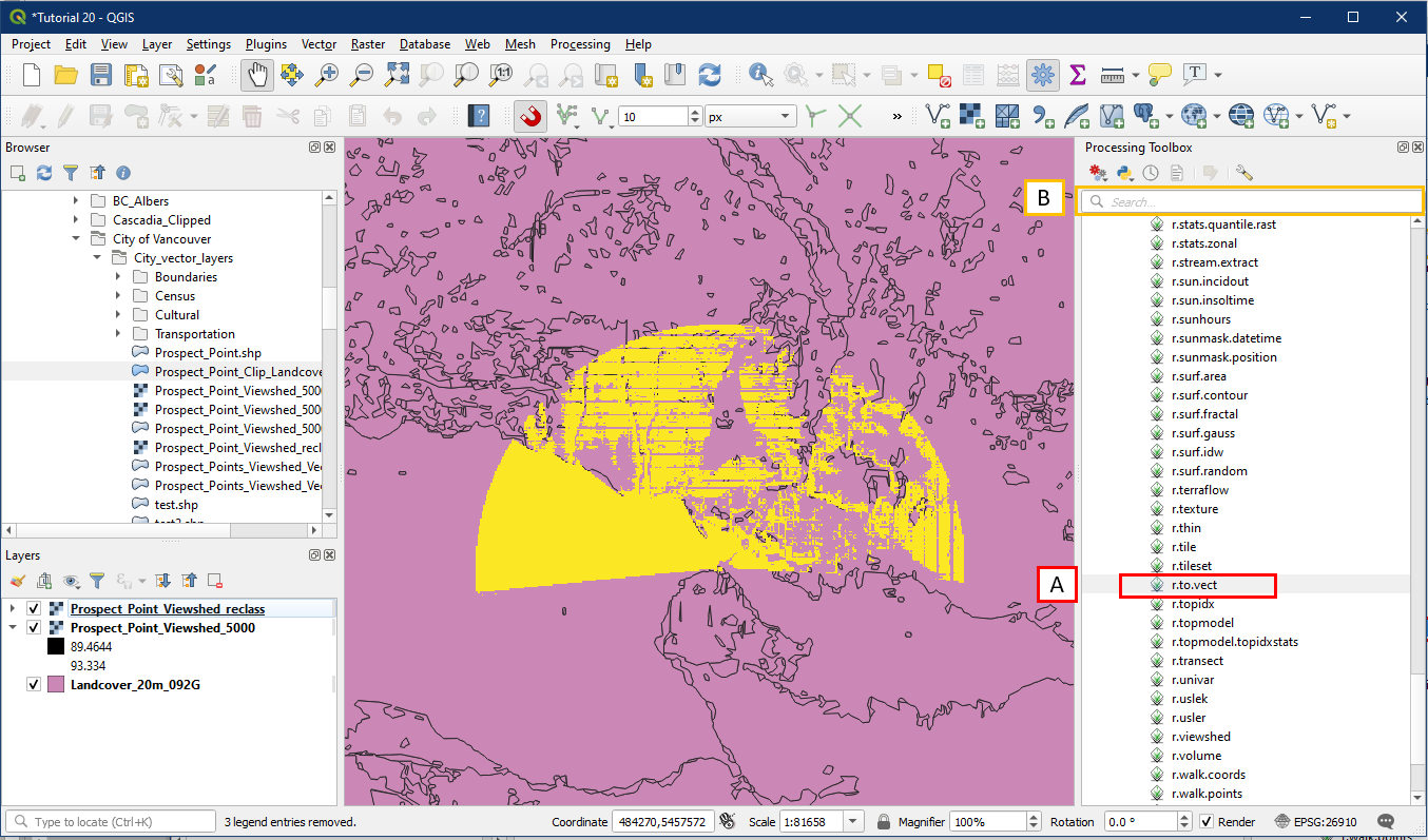
To convert from raster to vector, go to Processing Toolbox > GRASS > Raster > r.to.vect (A). Alternatively search for “r.to.vect” in the search box (B).

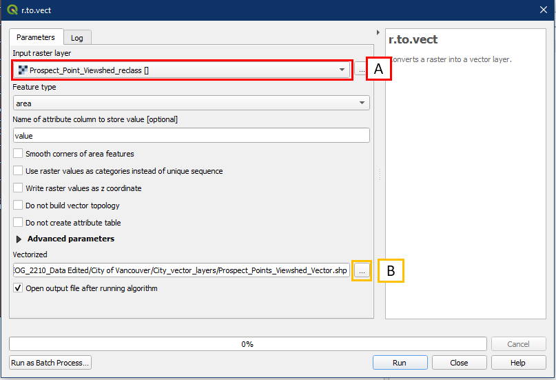
In the r.to.vect dialog window, choose the following settings:

1. For Input raster layer select the reclassified viewshed layer
2. Click the “…” to Save to File, specify a folder location and file name for the new vector viewshed layer

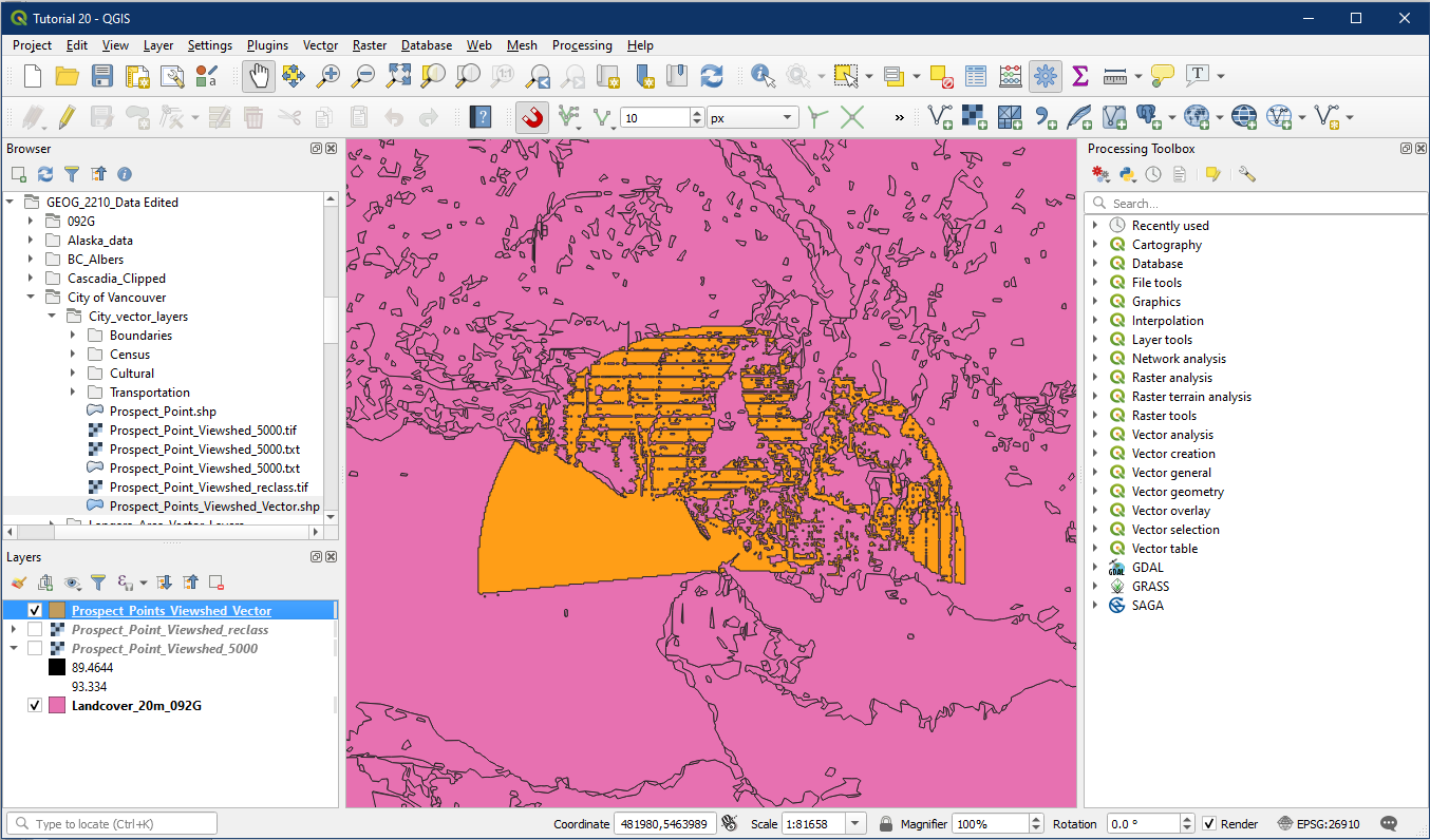
The converted vector viewshed layer will look something like this.

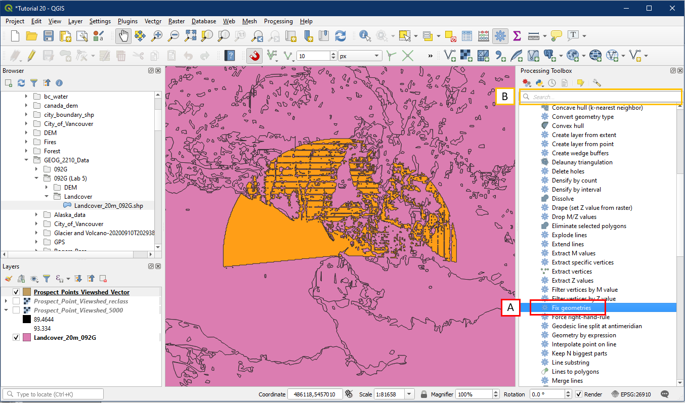
IMPORTANT: Currently, the raster/vector conversion tools produces vectors that have some geometry issues. So before moving onto the next step please run the Fix geometries tool. Go to Processing Toolbox > Vector geometry > Fix geometries (A). Alternatively search for it in the search box (B).

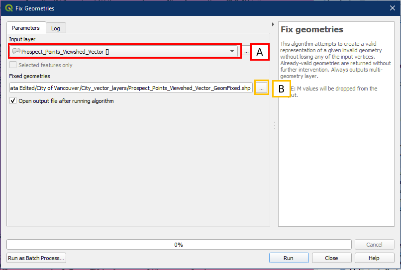
In the Fix geometries dialog window, choose the following settings:

1. For Input layer select your vectorized viewshed layer
2. Click the “…” to Save to File, select a folder location and file name for the geometry-fixed vector viewshed layer

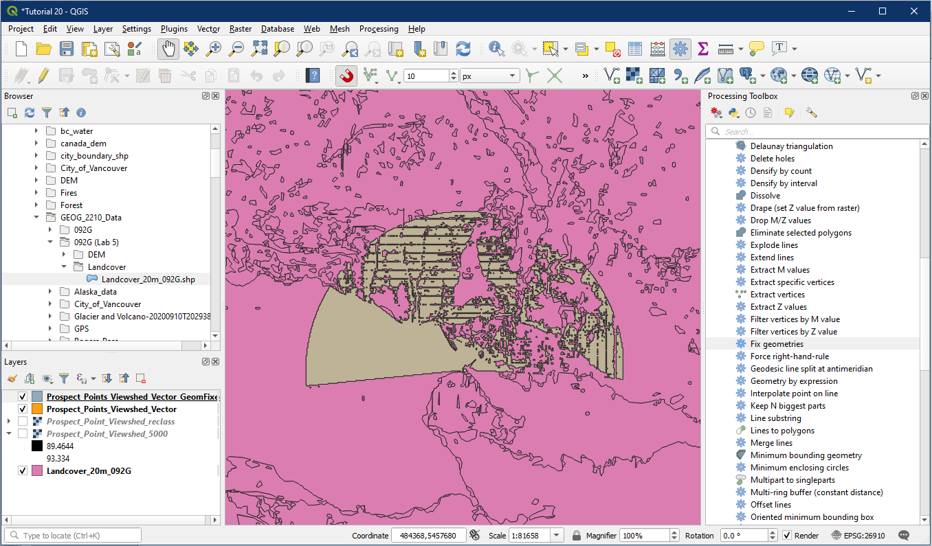
This new vector layer should now have no issues in the following Activity 2.

Activity 2: Vector Overlay

The next step is to extract or clip the landcover layer using the Prospect Point viewshed vector layer, in other words, we only want the portion of the landcover layer that coincides (or is the same) as the Prospect Point viewshed vector area.

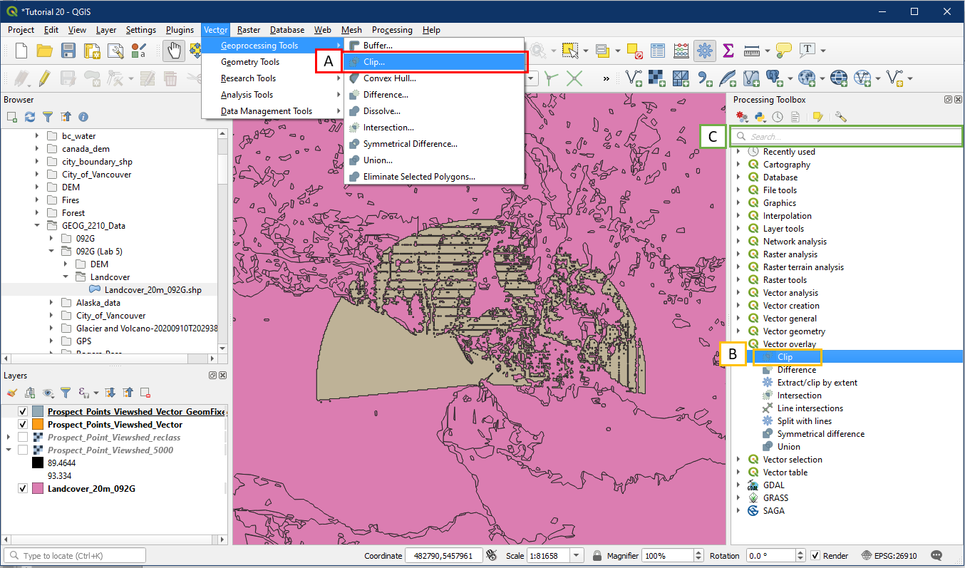
To access the clip tool, pick one of the following options:

1. Vector menu > Geoprocessing Tools > Clip
2. Processing Toolbox > Vector overlay > Clip
3. Search box

In the Clip dialog box, choose the following settings:

1. For Input layer choose the Landcover_20m_092G layer
2. For Overlay layer choose the geometry fixed vector viewshed layer from Activity 1
3. Click the “…” button to Save to File, select a folder location and file name for the clipped layer.

The clipped layer will have the outline shape of the viewshed vector layer, but the interior will contain the landcover details. Additionally, it’s attribute table will also contain the details from the landcover layer, which we will use later.

Activity 3: Vector to Raster

The best method for quantifying area and other geospatial statistics is often in a raster format. So we will take the clipped landcover vector layer from Activity 2 and turn it back into a raster layer so we can produce a report.

To do so go to the Processing Toolbox > GRASS > Vector > v.to.rast (A). Alternatively search for “v.to.rast” in the search box.

In the v.to.rast dialog window select the following settings:

1. For Input vector layer, choose your clipped landcover layer
2. For Name of column for ‘attr” parameter select the COVTYPE field
3. For Name of column used as raster category label also select COVTYPE
4. Within Advanced parameters, under GRASS GIS 7 region cellsize set it to 30 (same as our original DEM cell size)
5. Click the “…” button to Save to File, specify a folder location and file name for the new raster layer

The converted raster layer will look similar to this.

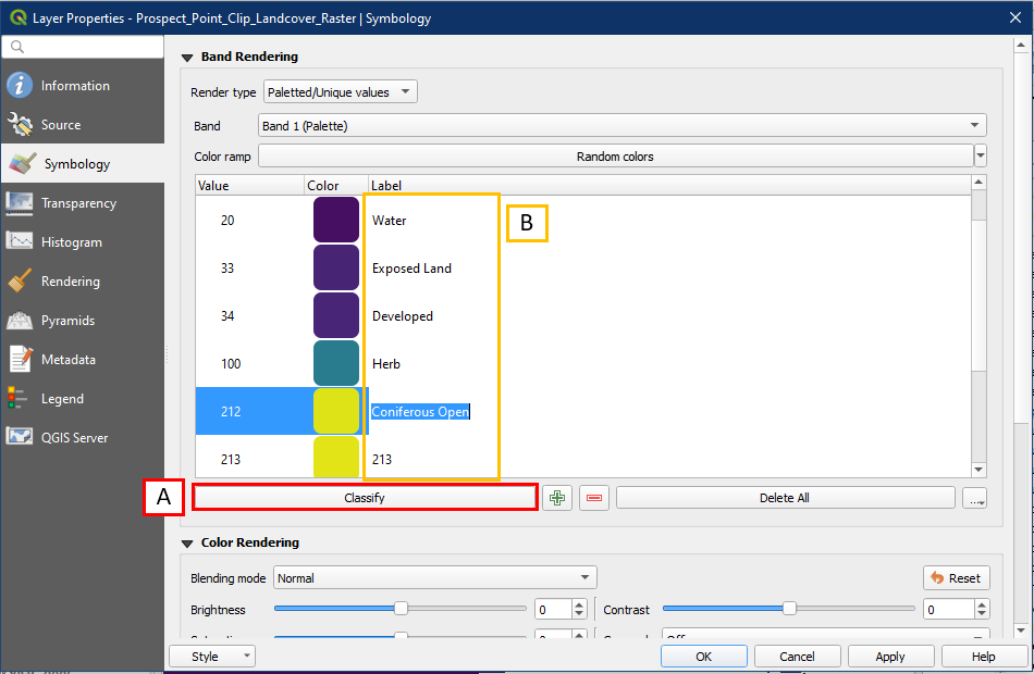
Go into the Symbology panel within the layer properties. Initially the layer will show lots of black/blank Symbology values, so click Classify (A) to remove them and to keep only the values found in the layer. Then rename the numbers under the Label column (B) based on the landcover classification codes shown below. Providing the actual name of each land cover type instead of numbers will be very helpful when making a map.

Next run the r.report tool and we can find the area for each landcover class. The down side is that the landcover classes are numerical codes, but we can refer to the class names from the code list above.

Save your project as Tutorial 20.