Raster based files are a form of continuous data. They store data in pixels or cells, although not every pixel was sampled to make the dataset; rather, the GIS uses forms of statistical algorithms/analysis to interpolate of neighbouring cells. This form use of geostatistics models the surface to estimate the values.

Here are some different methods for modelling surfaces. If you consider all of the different data that can be collected from a surface and the impossible task of being able to collect samples from every area on a surface (Earth) then you will understand the value of these interpolation techniques. Some examples of data monitored from surfaces: elevation, temperature, wind speed, humidity, gradient (slope), aspect, etc.

Simple methods:

• Nearest-neighbor interpolation here is a video explaining it
• Bilinear Interpolation
• Inverse distance weighed interpolation

More Advance Methods:

• Kriging

This tutorial will examine the use of continuous elevation data stored in raster format as a Digital Elevation Model (DEM). Not all cells were sampled and the unsampled cells are provided values through interpolation. There is enormous utility in the use of elevation data to analyze terrain. In this tutorial we will examine hillshades, aspect, and slope; which are all valuable when assessing or conducting terrain analysis.

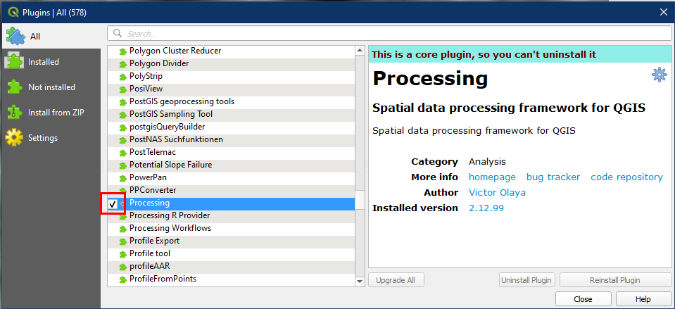
Before beginning the tutorials activities lets ensure that we have enable the Processing Toolbox in QGIS. To do so, first click Plugins > Manage and Install Plugins, and make sure that the checkbox for Processing is checked. Plugins are essential to the operation of QGIS and I suggest you spend some time investigating the various plugins and their functions, many will improve your GIS skills and make you a more efficient user.

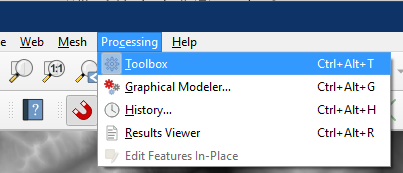
Now we can open the Processing Toolbox. Notice that the top menu bar now has the Processing menu. Click on it and select Toolbox.

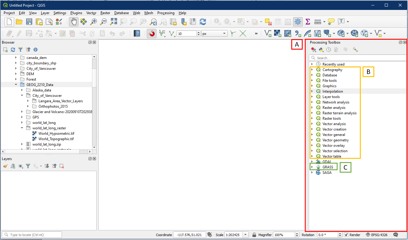
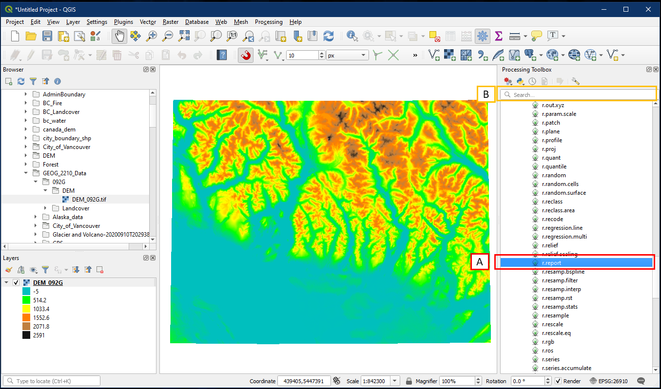
The Processing Toolbox panel (A) should now be displayed on your QGIS GUI. Within it, we will find all the QGIS tools available (B) within tool categories that has the QGIS logo. Additionally, we will use some tools from the GRASS toolbox (C). Grass GIS is a different open-source GIS software, but is supported by the same foundation of members of OSGEO. Hence the compatibility between the two GIS programs.

Activity 1: Reports

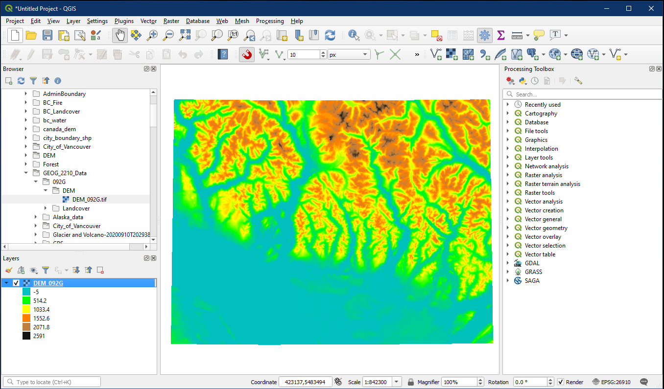
Open a new QGIS project and load the DEM_092G (locate file in Brightspace>Content>Labs>Lab 4) raster layer. The layer should be black and white by default, so change the colour based on tutorial 10 (Quantitative Raster Data section), but for Mode choose Continuous.

We want to create a basic text report via the r.report tool. In the Processing Toolbox select GRASS > Raster > r.report (A). Alternatively, search for “r.report” using the search box (B).

In the r.report dialog window, choose the following settings:

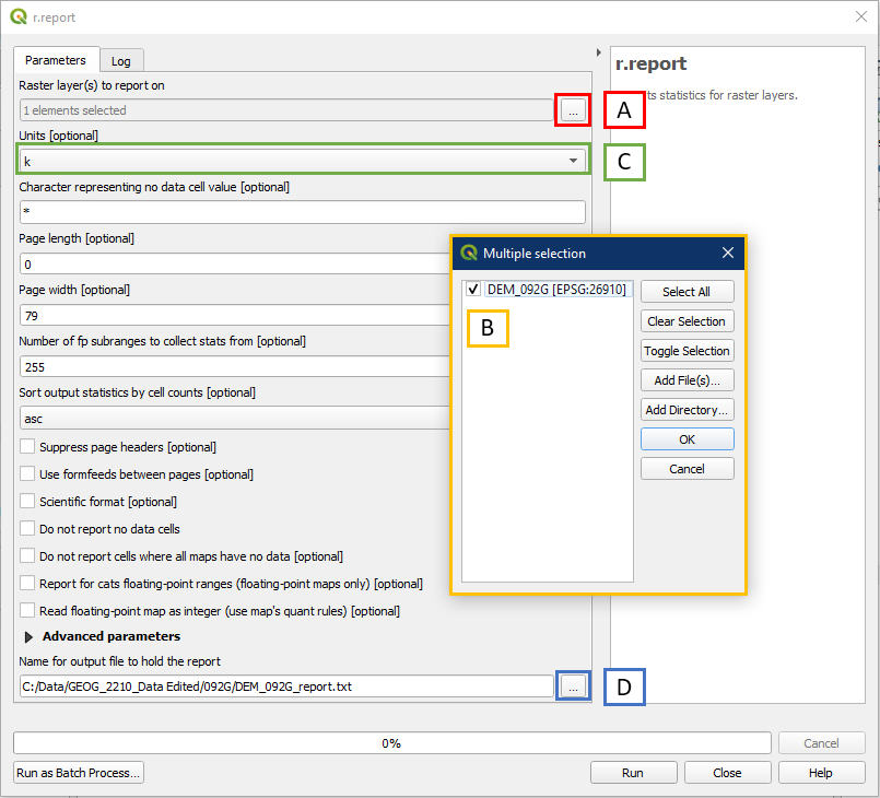
1. Under Raster layers to report on, click the “…” button to select the layer to report on
2. The Multiple selection window will appear, select the DEM_092G layer. Important: make sure you always select only the layer you are reporting on, multiple layers tend to produce weird results.
3. Under Units, select k (stands for kilometres). Alternatively you may wish to select me (stands for metres).
4. Click the “…” button to Save to File, choose a folder location and file name for the report text file

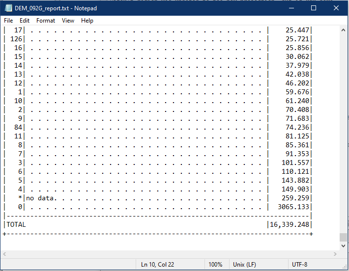
Browse to your folder location and open the report TXT file. It will contain information like raster extent, resolution (res) and the area for each pixel value.

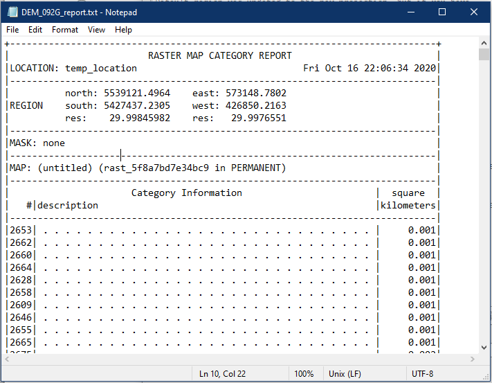
Scroll to the very bottom and we will see the total area covered by the raster file.

Activity 2: Hillshades

We will create a shaded relief layer from this DEM layer. There are several ways of doing so:

1. Go to the Raster menu button > Analysis > Hillshade. This is the simplest option, but the menu does not contain every single tool.
2. Alternatively, within the Processing Toolbox expand the Raster terrain analysis tools and select Hillshade. The Processing Toolbox is harder to navigate, but contains every single tool in QGIS.
3. Hint: you can also search for tools using the search box e.g. type in “hillshade” and selecting the Hillshade result. This is a good method once you become familiar with the tools.

Whichever method will open up the Hillshade dialog window. Within the window select the following:

1. Under Elevation layer, select the DEM_092G layer (it should be automatically selected if it was the only raster layer in your layer panel)
2. Select the “…” button to Save to File, select the folder location and name for the new shaded relief layer
3. Click Run, and close the window when it is complete

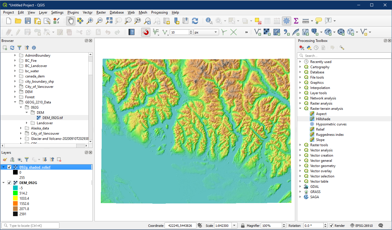
The shaded relief layer should look something like this.

Change the transparency of your shaded relief layer will resemble a similar effect from the earlier raster tutorials. This is a basic form of shaded relief map.

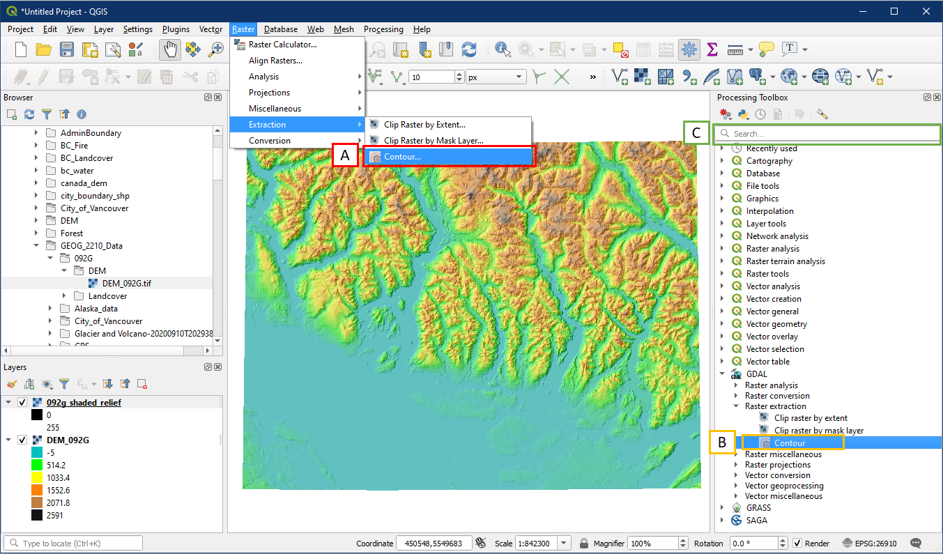
Activity 3: Contours

The DEM is a raster based data product but to improve understanding of the elevations Cartographers often use vector-based contour lines, the use of contour lines provides evidence for planning routes, construction, etc…

To create contours, pick one of the following options:

1. Raster menu button > Extraction > Contour
2. GDAL toolbox > Raster extraction > Contour
3. Search for “contour” and selecting the Contour result

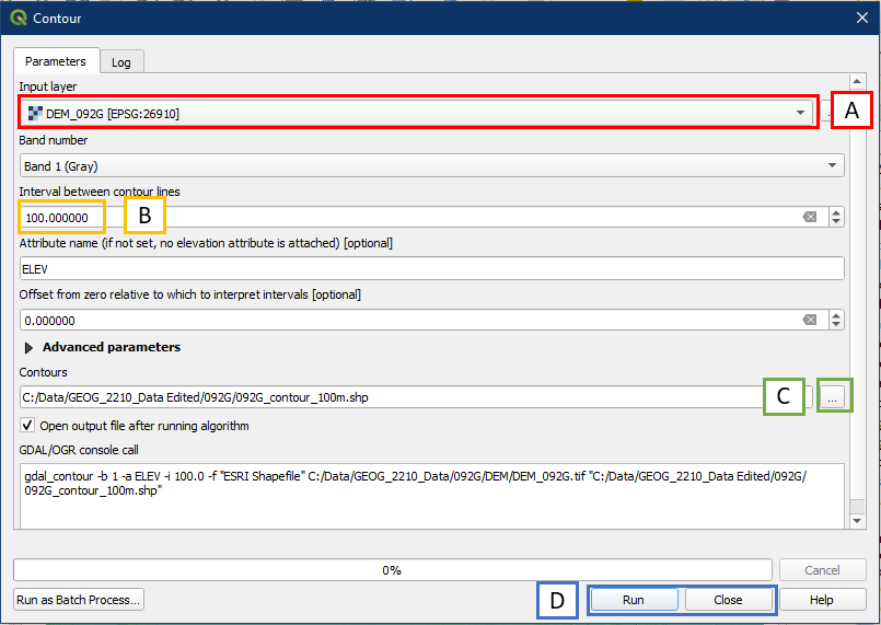
Within the Contour dialog window, choose the following settings:

1. Select the DEM_092G layer. A common mistake is selecting the wrong raster layer (e.g. hillshade instead of the DEM) which will not have the desired result.
2. Set a contour interval of 100 m
3. Click the “…” button to Save to File, choose a folder location and file name
4. Click Run, and Close once the task is done.

The default colour may be difficult to see. Zooming in and changing the contour to black lines may help. The contours along with the layers DEM and hillshade produces a shaded relief contour map.

Right clicking on the contour layer > Open Attribute Table and we see that each feature/line has as corresponding elevation value under ELEV. This will be useful if this layer ever needs to be labelled.

Activity 4: Aspect

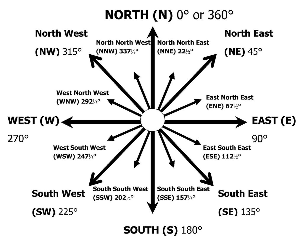
Aspect is the compass direction that a topographic slope faces, usually measure in degree from north. Humans are interested in slope aspect for a variety of reasons including some real-world examples:

1. Farmers seed crops depending on the amount of incoming solar radiation and aspect data.
2. Ecologists study aspect and microclimate for biodiversity.
3. Recreational planners study slope direction to prevent avalanches.

To create an Aspect layer, pick one of the following methods to open the Aspect dialog window.

1. Raster menu button > Analysis > Aspect
2. Processing Toolbox > Raster terrain analysis > Aspect
3. Search for “Aspect” in the search box

In the Aspect dialog window select the following settings. Note that the dialog window may slightly different based on which method you chose above, but the input and output are the same.

1. For Input layer select DEM_092G. Again a common error is not selecting the DEM layer in this box.
2. Click the “…” button to choose Save to File, choose a folder location and file name for the new aspect layer
3. Click Run. Once the tool finishes click Close.

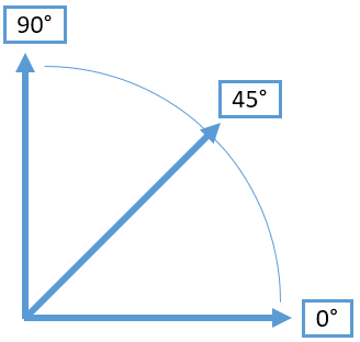
The aspect layer will look like something like this. Notice how in the layer Symbology, the values range from 0 to 359.9, representing the 360 degrees on a compass.

Activity 5: Slope

Slope is an expression of incline, gradient, or incline of a hill. Often measured as a slope angel (Euclidean geometry) or as a percentage. Humans are interested in slope for a variety reasons. We often classify slopes like this or are interested in the angle of repose (slope stability) for different materials. Understanding the different slopes can provide insight into a wide variety of issues like: avalanches, landslides, road construction, sand castle building etc…

To create a slope layer, choose one of the following methods to open the Slope dialog window.

1. Raster menu button > Analysis > Slope
2. Processing Toolbox > Raster terrain analysis > Slope
3. Search for “slope” in the search box

In the Slope dialog window, choose the following settings. Note that the dialog window may slightly different based on which method you chose above, but the input and output are the same.

1. For Elevation layer choose the DEM_092G raster layer
2. Click the “…” button to Save to File, choose a folder location and file name for the new slope layer.
3. Click Run, and click Close when the tool finishes running.

The slope layer will look something like this. Notice that in the layer Symbology it will have values ranging from 0 (flat) to 90 degrees (vertical). This this specific case the maximum slope is 79 degrees within the layer extent.

Great work. Feel free to save your QGIS Project e.g. Tutorial_17.