Coordinate Reference Systems

Coordinate Reference Systems (CRS) are divided into two main categories: Geographic Coordinate Systems and Projected Coordinate Systems.

Geographic Coordinate Systems treat the world as a sphere and uses latitude and longitude (degrees) as the unit of measurement.

In contrast, Projected Coordinate Systems projects the world onto a flat map, and uses metres or feet as the unit of measurement. The various map projections we will talk about in class are all Projected Coordinate Systems.

To read more about Coordinate Reference Systems from the QGIS website: Coordinate Reference Systems.

QGIS also has a page on working with Projections.

Activity 1: Different CRSs

The ability to set a CRS and understand the differences is crucial and possibly one of the most difficult of all GIS related topics.

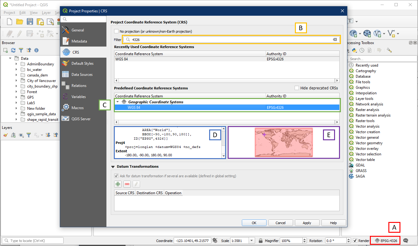
Open a blank QGIS project. Click on the Project CRS button (A) on the bottom right to open up the CRS settings within Project Properties. It displays the current CRS for this project (e.g. EPSG:4326). Within the filter box (B), search for 4326. WGS 84 EPSG:4326 remains the results box (C), click to select it. Notice how this CRS is found under the category Geographic Coordinate Systems.

In the CRS details section (D) scroll down and you will notice that the Extent: -180.00, -90.00, 180.00, 90.00. This means the extent of the geographic coordinates are 180 degrees west, 90 degrees south, 180.00 degrees east, and 90.00 degrees north. West and south degrees are displayed as negative numbers. This extent covers the entire world, which we can see in the overview map (E).

Press OK, and this will set the project CRS to EPSG:4326.

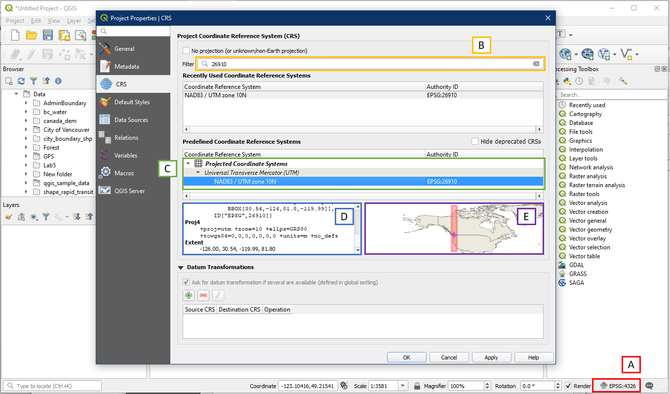
Open the Project CRS properties again (A). This time in the search box (B) search for 26910. NAD82 / UTM zone 10N EPSG:26910 should remain in the box (C), select it. Notice how this CRS is found within the category Projected Coordinate Systems.

In the CRS details section (D) scroll down and notice that the extent is smaller than the EPSG:4326 extent. The map (E) also visually shows that this CRS covers a much smaller area. Note that the area outside this extent can still be displayed using this CRS, just not accurately. You will also notice that the projection = UTM Zone 10, Ellipsoid = GRS80, and Units = Metres.

Press OK to set the project CRS to 26910.

Activity 2: Testing On the Fly Functionality

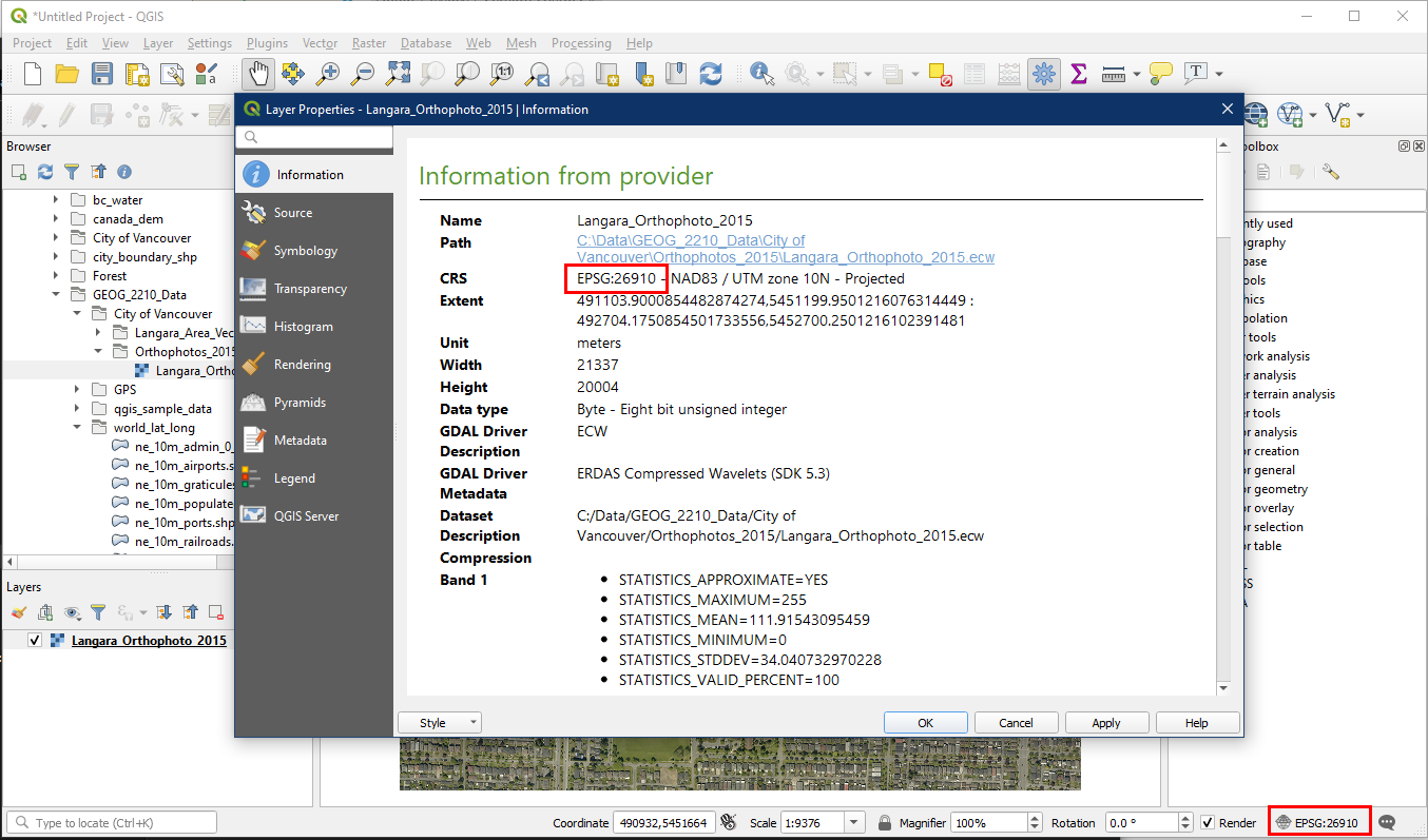
Keep your project in EPSG:26910. In the Browser panel locate the Langara_Orthophoto_2015 layer from the City_of_Vancouver folder, and add it onto the map, it should open with no issues.

If you right click on the Langara_Orthophoto_2015 layer and open Properties, you can see that this layer has the same CRS as our project.

Now go to the Browser panel and locate the layer ne_10m_admin_0_countries in the world_lat_long folder and add it to the map. The Select Transformation window will appear, because the layer uses a different CRS than the project. Since QGIS has On the Fly capability, this is fine. Simply press OK.

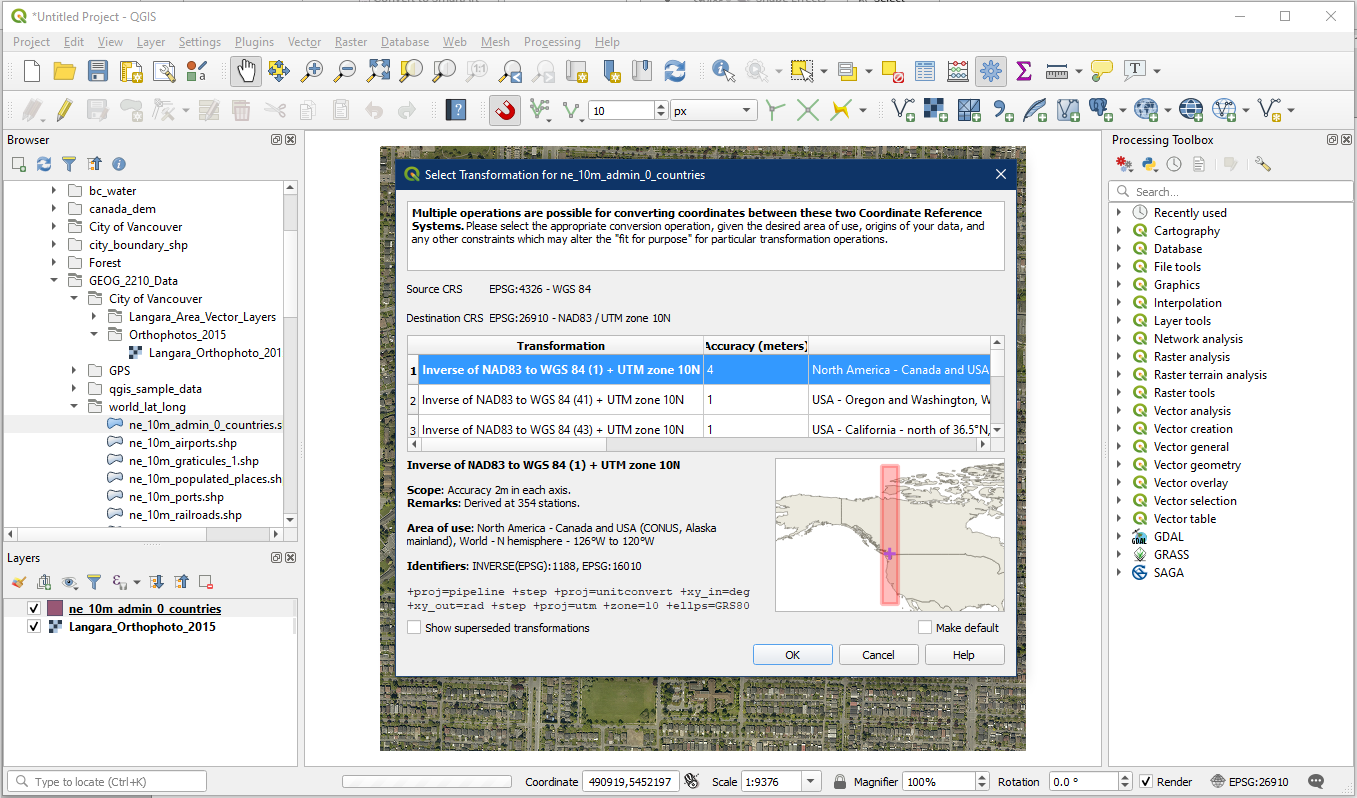
Rearrange the layers so that Langara_Orthophoto_2015 is on top within the Layers panel, and zoom out. You will be able to see the Langara golf court within the context of the world.

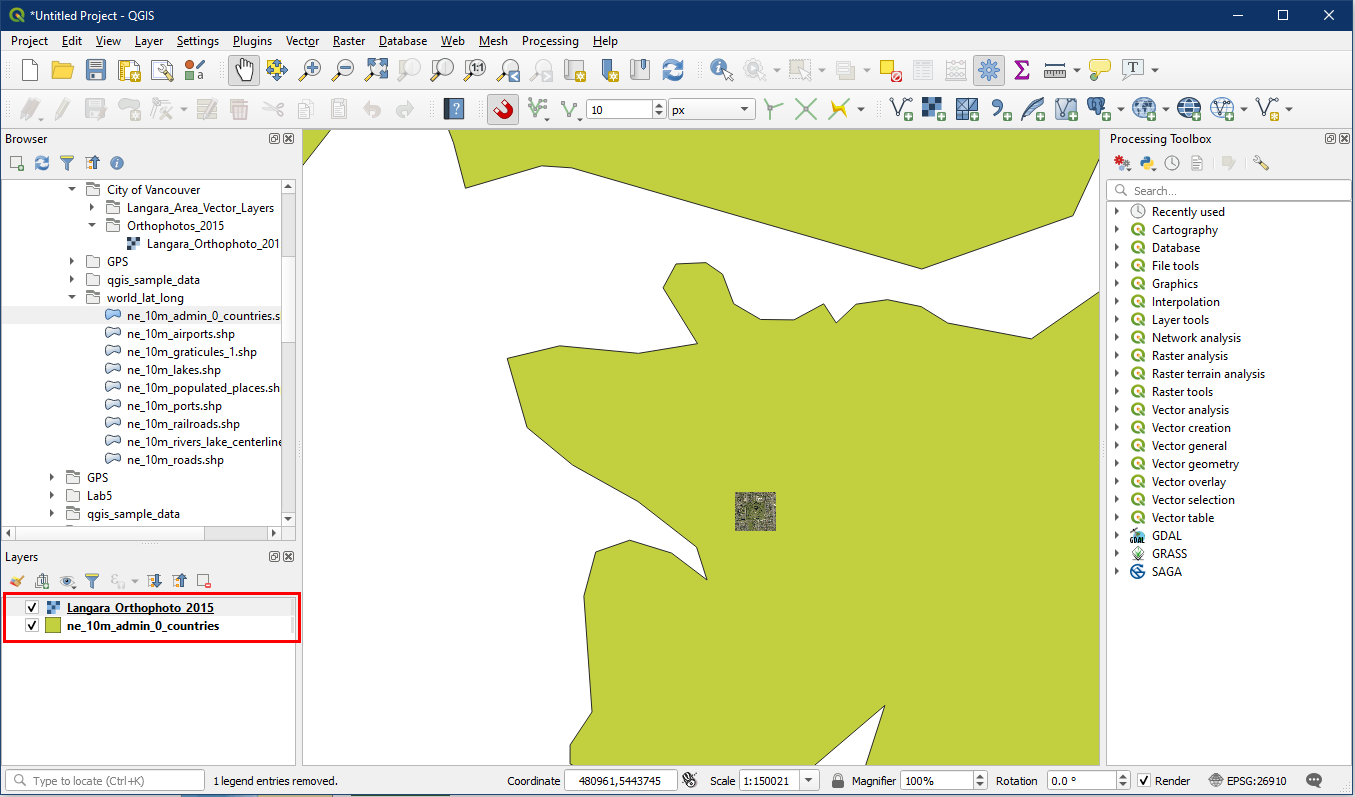
Everything appears to work fine. However if you right click on ne_10m_admin_0_countries and open Properties, you will see that the layer CRS (4326) is different than the project CRS (26910). Having layers in different CRS will result in problems when using GIS analysis tools, so we will be learning how to reproject layers next.

There is no need to save this project.

Reprojecting Layers

Why do we reproject? Here is an excellent explanation from GIS:Stack Exchange:

Here are some useful links to help understand different projections:

• Vox video on projections
• Interact with projections
• Mercator tool
• Mike Bostock Map Transitions
• Mercator Puzzle

Activity 3: Reprojecting Vector Layers

In this example we will reproject vector layers from a Geographic Coordinate System into a Projected Coordinate System using the Export > Save as function.

Open a new project. For this activity the project CRS does not matter, since we are only interested in the layer CRS.

In the Browser panel find the world_lat_long folder and add the following layers to the map, and arrange them in this order.

1. ne_10m_populated_places
2. ne_10m_roads
3. ne_10m_admin_1_states _provinces

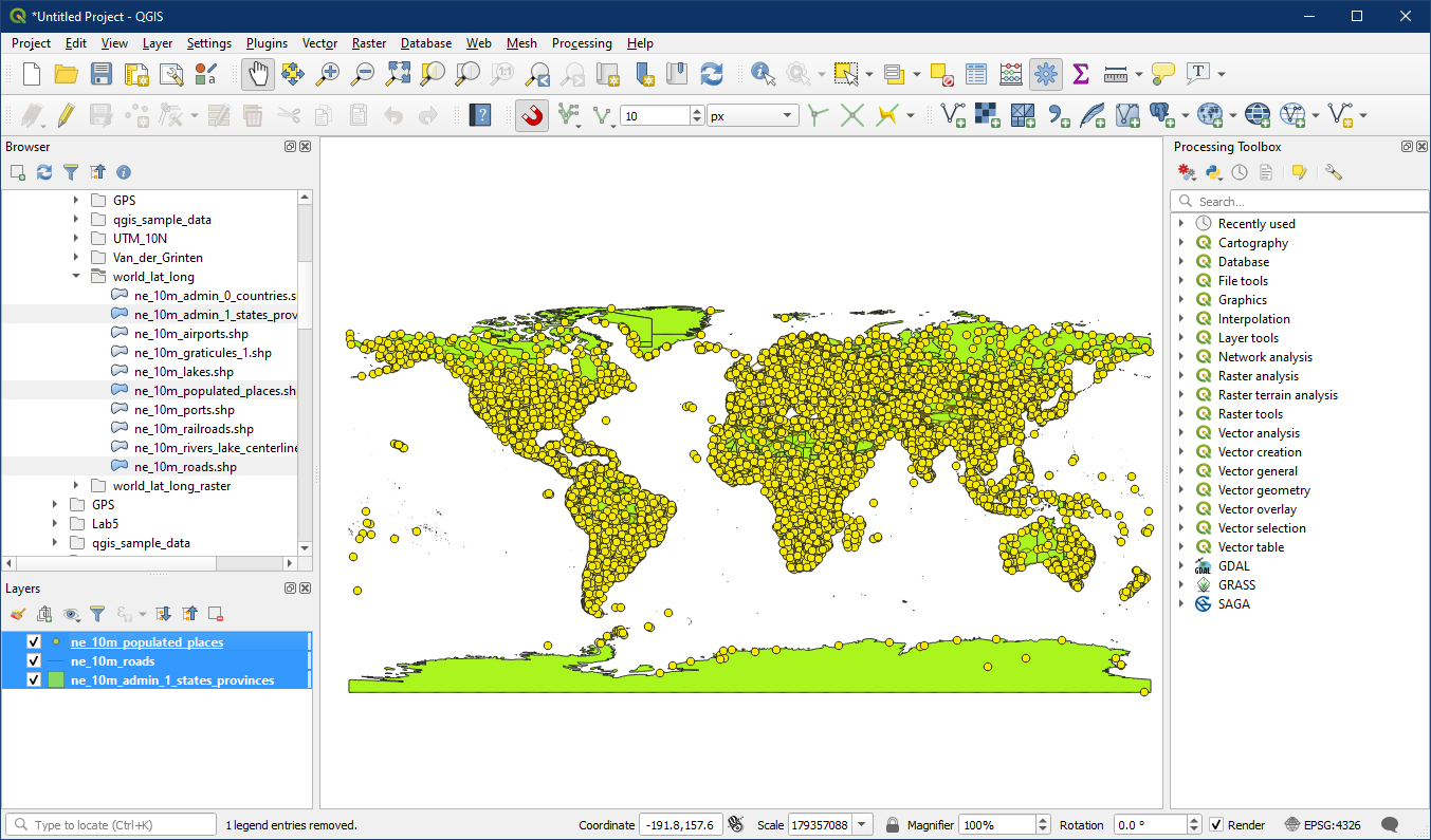
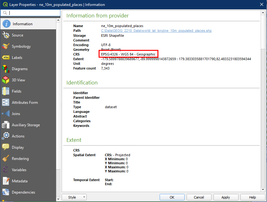
If we right click on any of these layers and look at its Properties, we will see that these layers all have EPSG:4326, a Geographic Coordinate System.

We now want to save these layers as a new set of layers with EPSG:3005, which is a Projected Coordinate System. EPSG:3005 is also known as BC Albers, a common map projection used for the province of BC and surrounding areas.

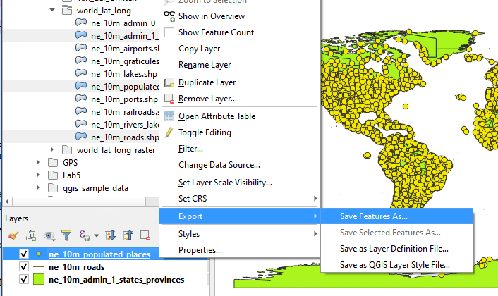
To do so, right click on ne_10m_populated_places in the Layers panel, and select Export > Save Features As.

In the Save Vector Layer window, set the following:

1. Within Format choose ESRI Shapefile
2. Click the “…” button to pick a folder location and file name for the new layer. For example create a new folder called “BC_Albers” and call the layer Populated_Places_3005 (number to indicate the CRS)
3. Click the Select CRS button which will open the Coordinate Reference System Selector
4. In the CRS Selector window, search for 3005 (D1). Select NAD83 / BC Albers EPSG:3005 from the window (D2). Click OK (D3).
5. Click OK in the Save Vector Layer window

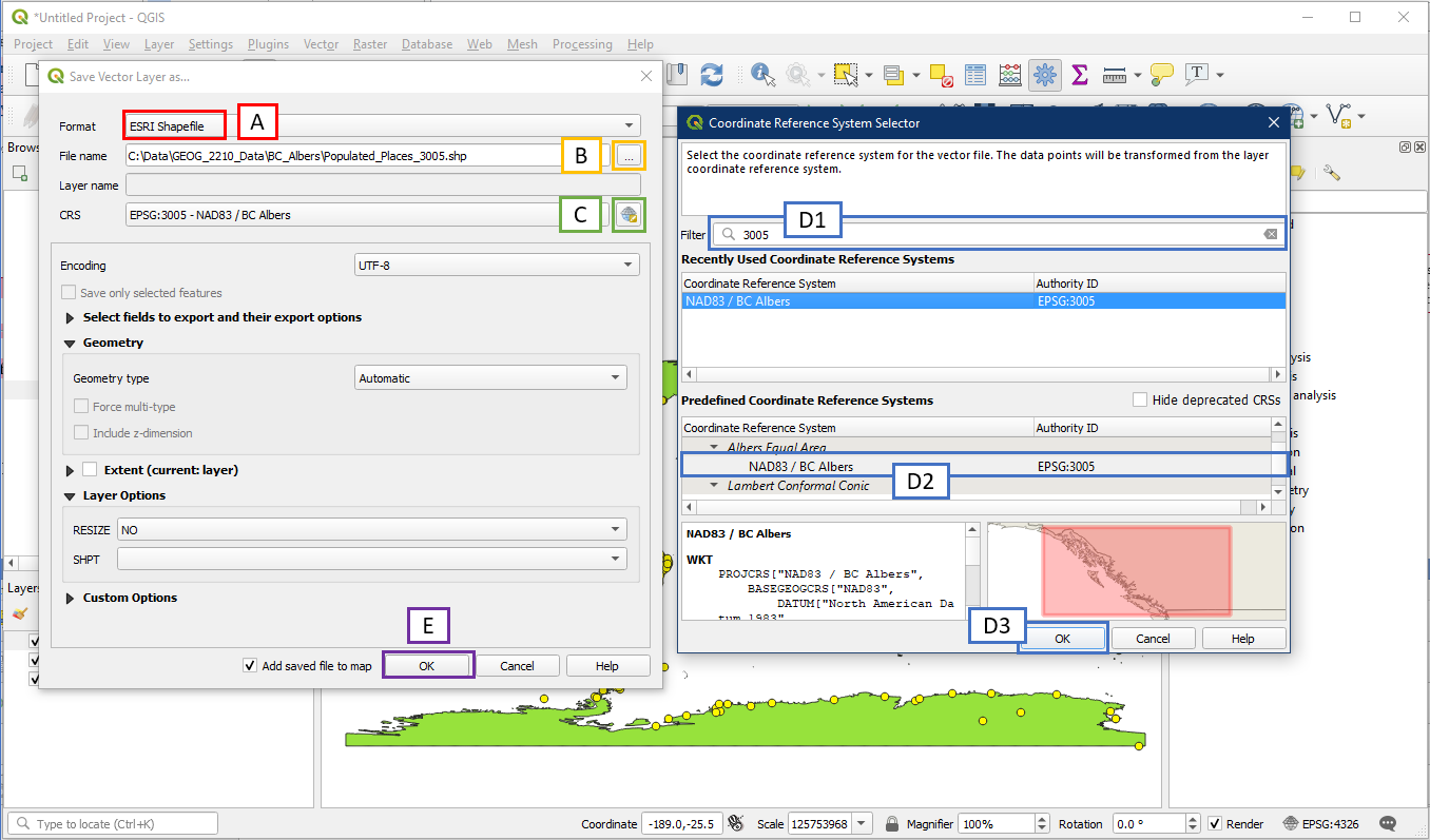
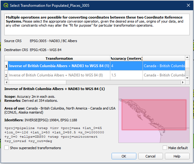
The Select Transformation window may appear. Simply click OK. This happens when the layer has a different CRS than the project, which makes sense since our new layer should be different.

The new Populated Places layer will now appear. It will look the same as the original ne_10m_populated_places layer but they will have different CRS in the layer properties.

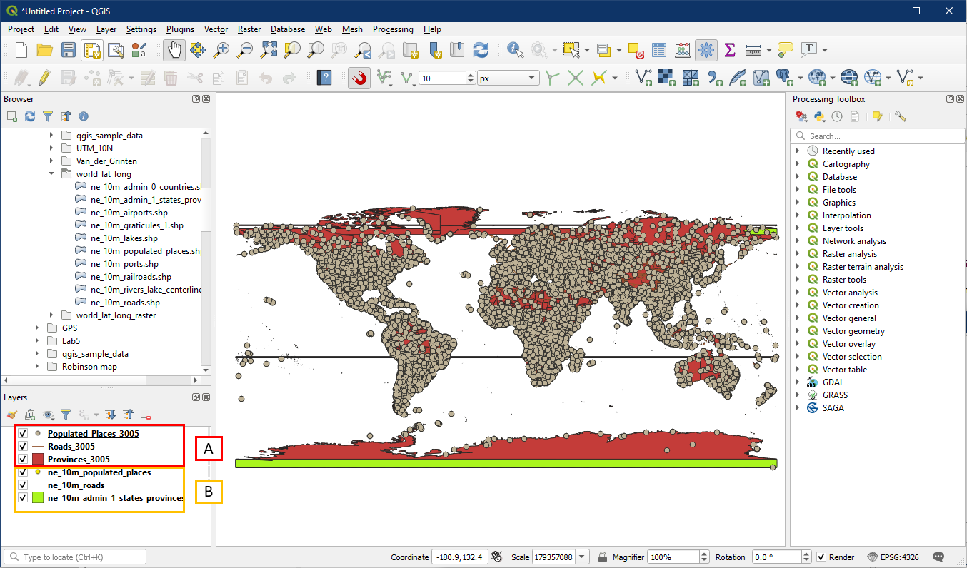
Repeat the Export > Save Layer As process for the road and countries layer and you will end up with three new layers with EPSG:3005 (A) in addition to the three original layers with EPSG:4326 (B). Note that the new states/provinces layer will look distorted, this is okay since it will look fine if displayed in the new EPSG:3005 projection.

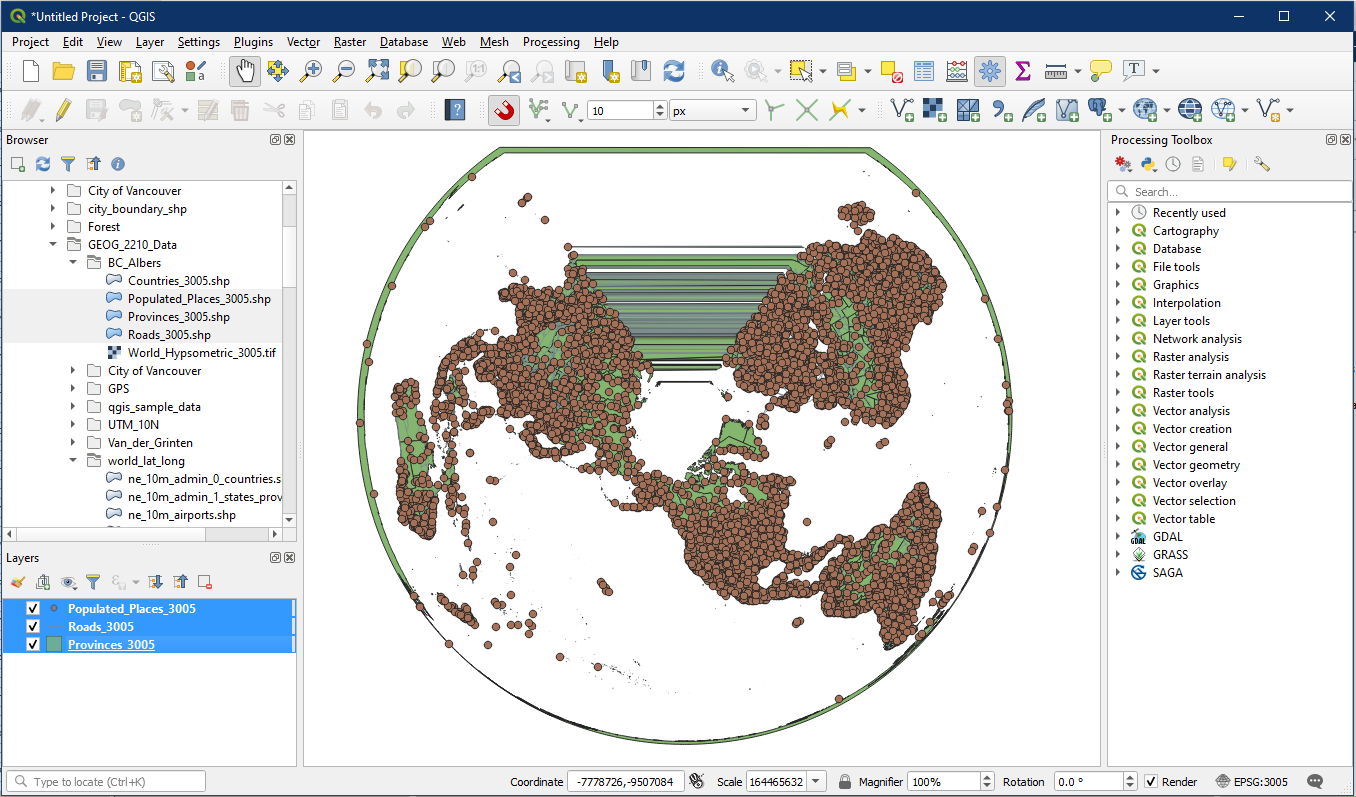
You can now close the project (no need to save). Open a new blank QGIS Project. We want this project to have the BC Albers projection. So click the Project CRS button in the bottom right corner (A). Search for 3005 (B) and select NAD83 / BC Albers EPSG:3005 (C). Click OK. Alternatively, you can skip this step if adding the layer into a blank project since QGIS will change the Project CRS to match the first layer it loads.

Locate the three EPSG:3005 layers we created earlier and add them to the map. Since the layers have the same CRS as the project, no additional messages will appear. Notice how most of the world outside of North America is highly distorted. This is because EPSG:3005 (BC Albers) is made display the province of BC, so areas will become increasingly distorted farther away from this focus area.

If we zoom into western Canada, the BC coast will look much better. Different CRS projections suit different areas, and creating regional maps will usually require selecting the appropriate projection.

Save this project as Tutorial_13.

 

Activity 4: Reprojecting Raster Layers

Reprojecting Raster layers is very similar to the process for vector layers; however, a few small differences exist. Raster layers exhibit continuous data vs. the discrete data of vector layers. This continuous data is formatted in pixels and thus when reprojecting or transforming from one projection (CRS) to another there are often constraints on the transformation process due to data types and size. Integers provide the greatest freedom when transforming.

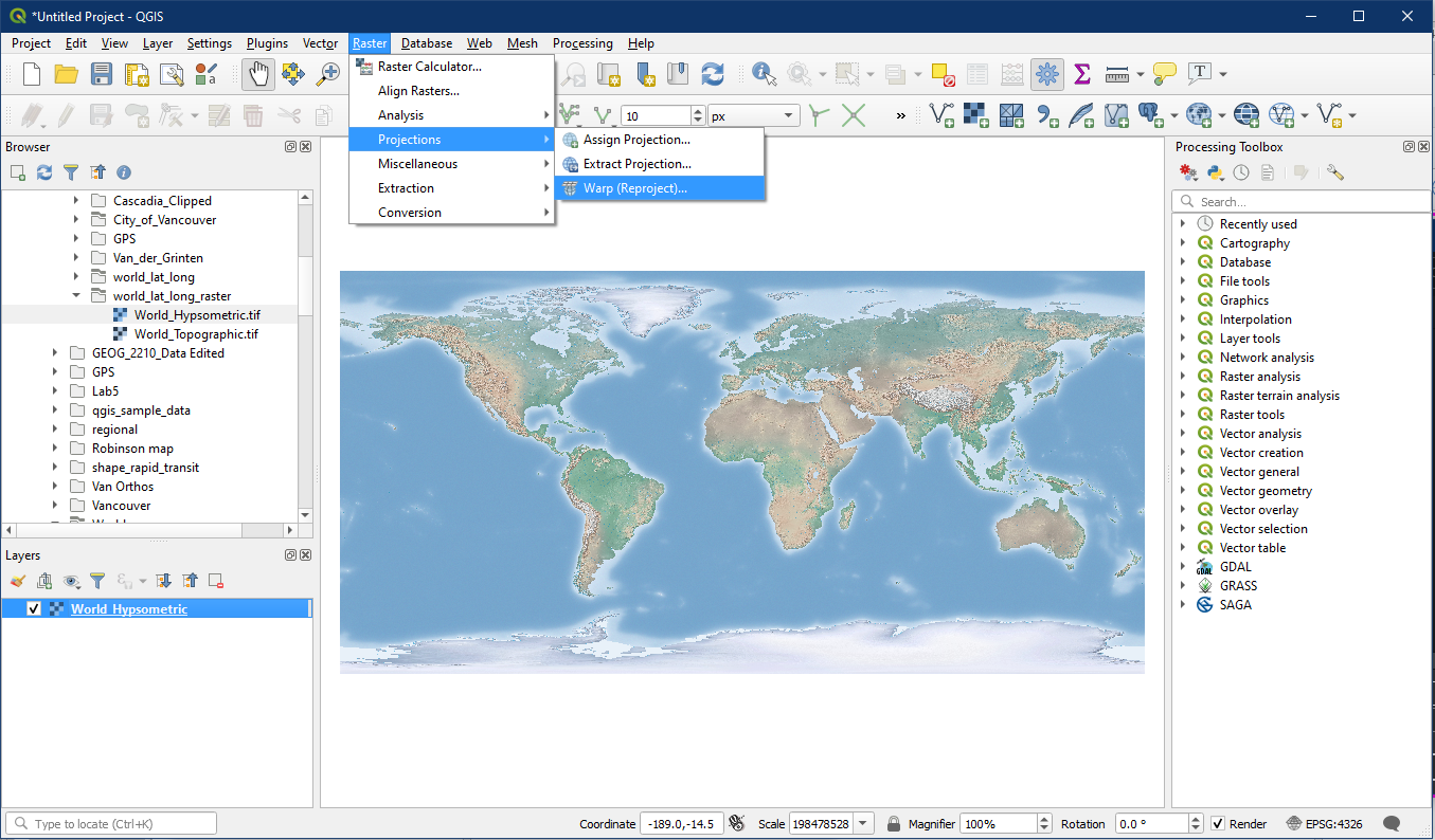
Open a new project and add the World_Hypsometric raster layer to the map. On the top menu select Raster > Projections > Warp (Reproject).

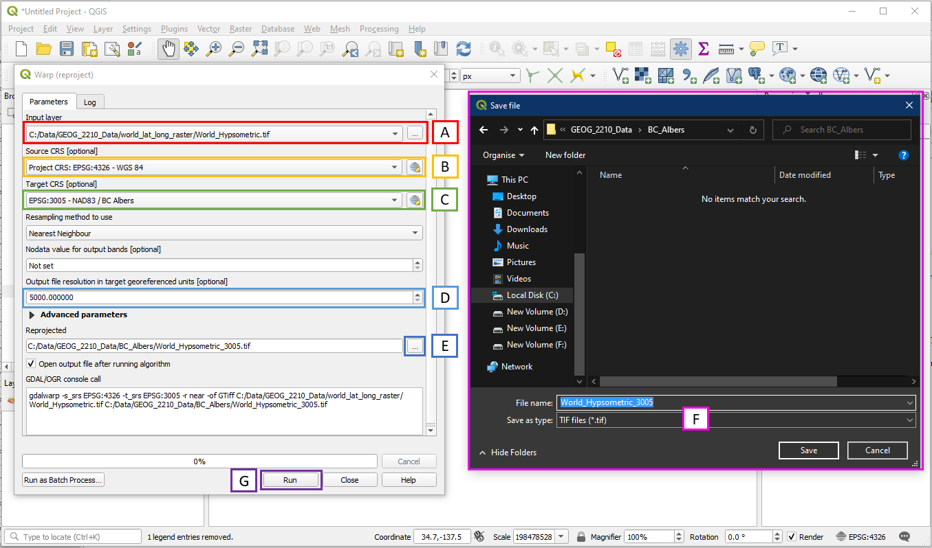
In the Warp (reproject) window, set the following:

1. Select the World_Hypsometric.tif raster layer in the Input Layer box. Alternatively use the “…” button if the layer is not present in the current project.
2. Source CRS is the CRS of the input layer, which we know to be EPSG:4326. You may need to use the globe button to select the CRS if it is not in the drop down menu
3. Target CRS is the CRS we want to reproject into, which in this case is EPSG:3005
4. Due to the nature of raster files, we want to specify a desired output raster resolution. For a map of this extent 5000 m is an acceptable resolution.
5. Click the “…” button and choose Save to File in order to select a folder location. Do not hype the file name into the box since it may save as a temporary layer
6. In the Save file window, choose a folder location and file name. For example save in the BC_Albers folder and name the file World_Hypsometric_3005. Also make sure to save as a TIF file type. Click Save.
7. Click Run. It may take a while to process.

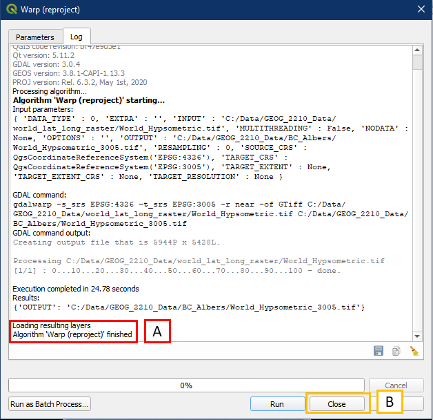
When completed, the Warp (reproject) window will not close by itself. The log will say that the Algorithm is finished (A). Click Close (B) when this happens.

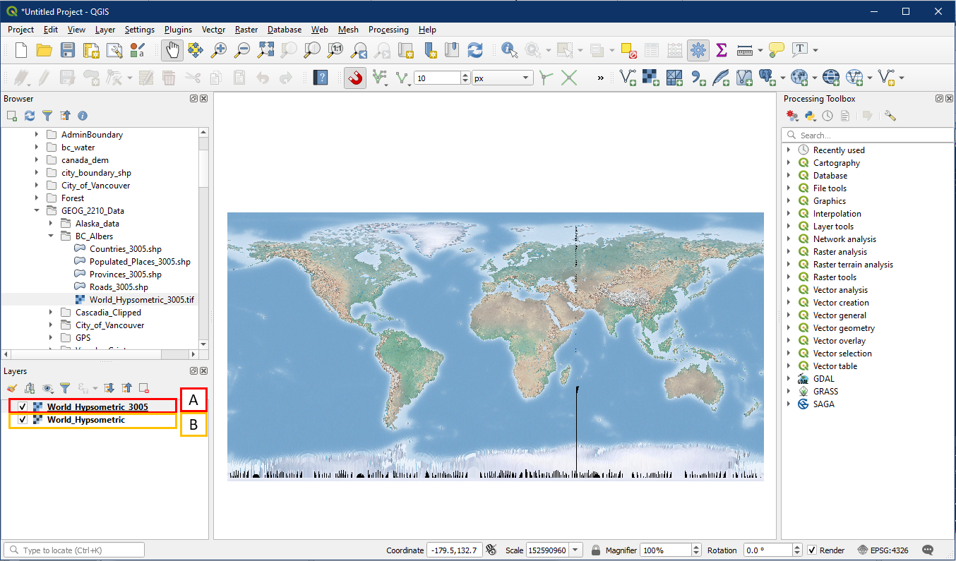
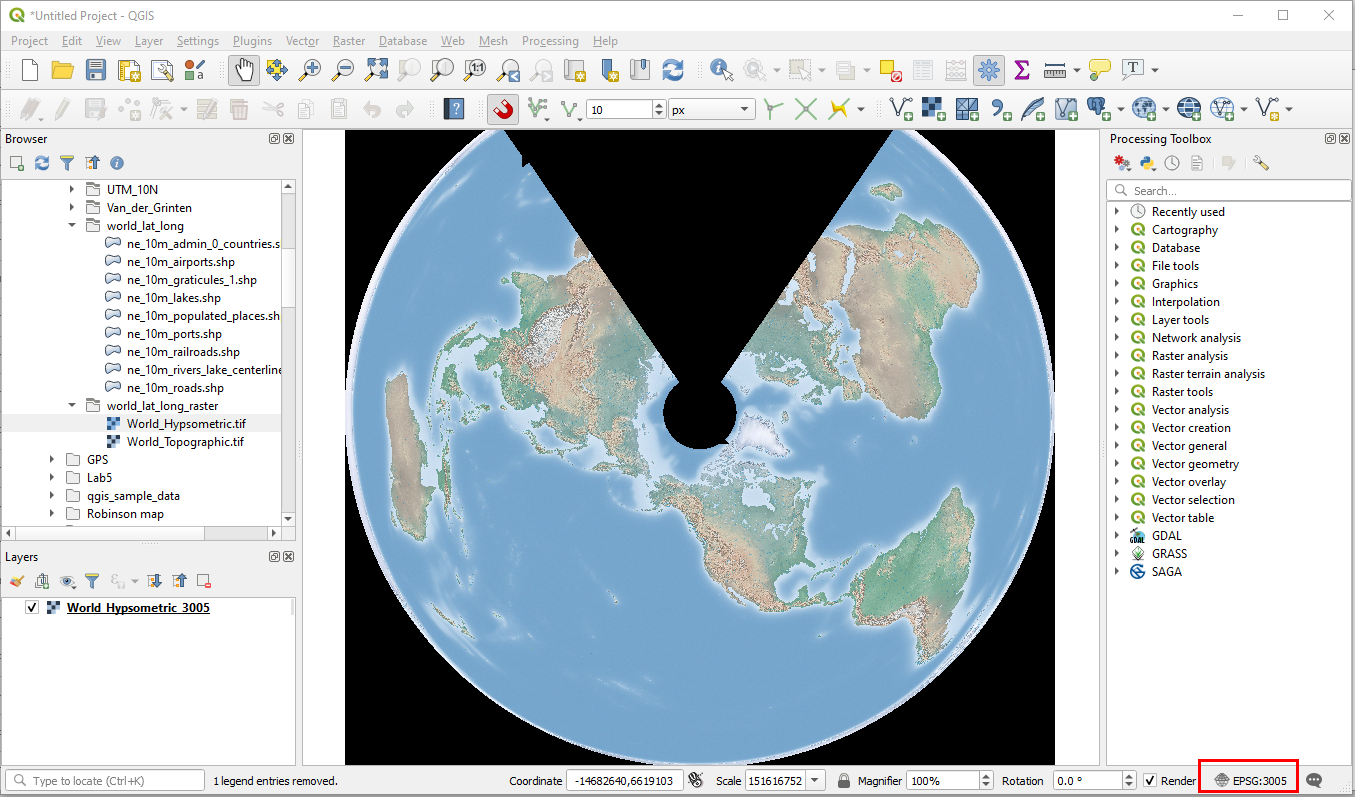
The new EPSG:3005 layer (A) will be added to the Layers panel on top of the original EPSG:4326 layer (B). However we can’t see the different right now because the project is still in the original EPSG:4326.

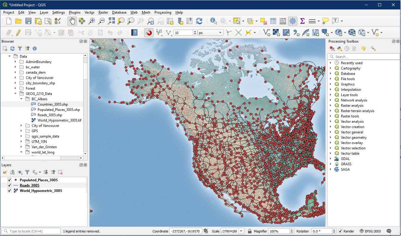
Open a new project and set the project CRS to EPSG:3005 in the lower right corner. Add the World_Hypsometric_3005 layer and see how the layer actually looks. Notice BC (the area meant for this projection) is displayed nicely while the rest of the world is heavily distorted.

You can now add the reprojected vector layers on top and they will be in the same projection.

Great work! Now you can reproject both vector and raster data.