It is appropriate at this point to briefly review the two fundamental data structures used for GIS data: vector and raster.

As you have seen in previous tutorials, the vector data structure uses points, lines and polygons (primitive objects) to represent spatial entities. Attribute information for the entities is stored in a separate attribute database that contains records that are linked to each spatial entity. In simple terms, the points, lines and polygons show where a feature is, and the attribute database describes the characteristics of the feature (read more about vector data in the QGIS reference manual).

In a raster data structure a geographic space is represented by a two dimensional (2D) gridded array (rows and columns) of cells. Each cell in the grid represents a rectangular (usually square) area of a specified length and width within that geographic space. The attribute value stored in the cell describes a characteristic of the space represented by the cell (see the general discussion on raster maps in the QGIS reference manual). QGIS is one of the few GIS applications that also supports three dimensional (3D) raster structures, but the use of these will not be covered in this series of tutorials.

This tutorial is intended to illustrate some fundamental raster layer concepts.

Activity – Displaying Raster Layers

Raster Symbology

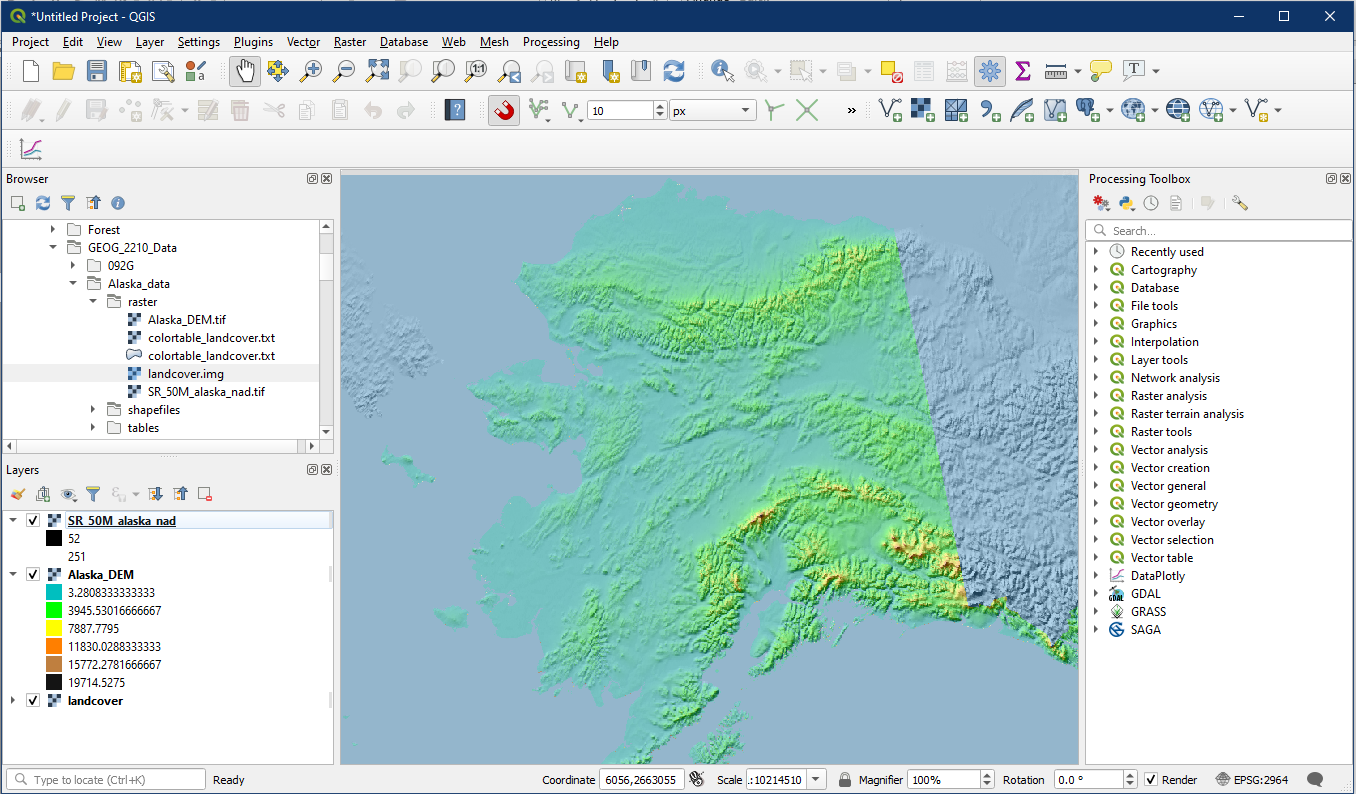
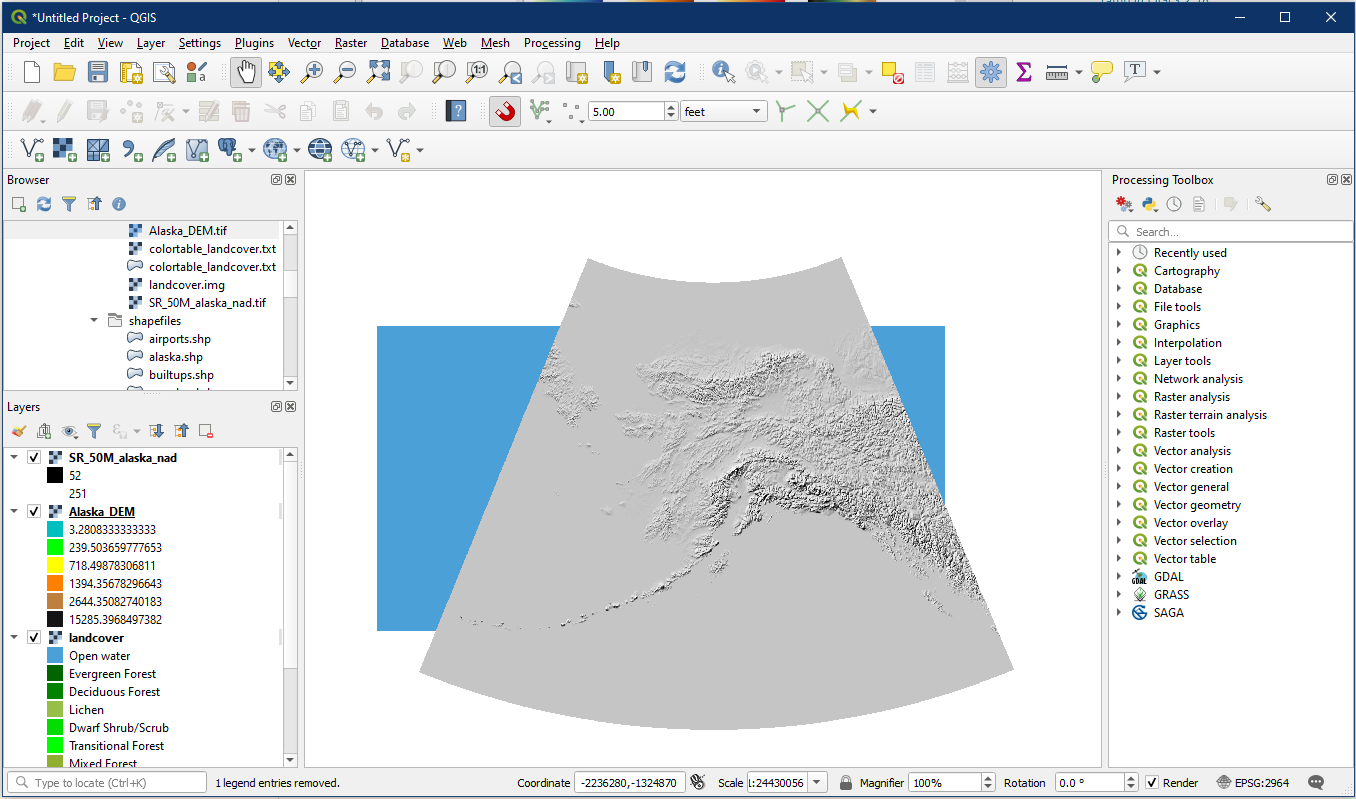
Open a blank QGIS map and add the following raster layers, found in the raster folder within Alaska_data:

• Alaska_DEM
• landcover
• SR_50M_alaska_nad

The attribute values in the landcover map layer would be considered qualitative data. In terms of measurement level, landuse/landcover categories are a nominal level of measurement. It is also possible for a raster layer to contain quantitative data, where the attributes are measured at the interval or ratio level of measurement. The Alaska_DEM elevation layer is an example of a raster layer containing quantitative data. The attribute values in the cells are elevation (feet) above sea level. Elevation above sea level is a measurement on the ratio level.

Qualitative Raster Data

Many landcover or nominal raster data formats will come with classifications that can be imported if they are not already found within the metadata or attribute data of the raster files. Unfortunately this landcover layer file does not have attributes other than the colour table attached. However a little research will yield the file perhaps. This is often the issue with data, the metadata is incomplete which compromises the dataset utility.

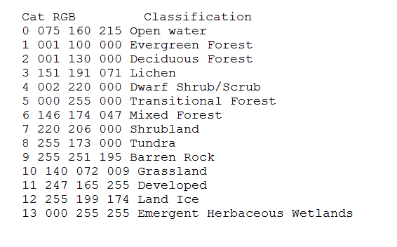
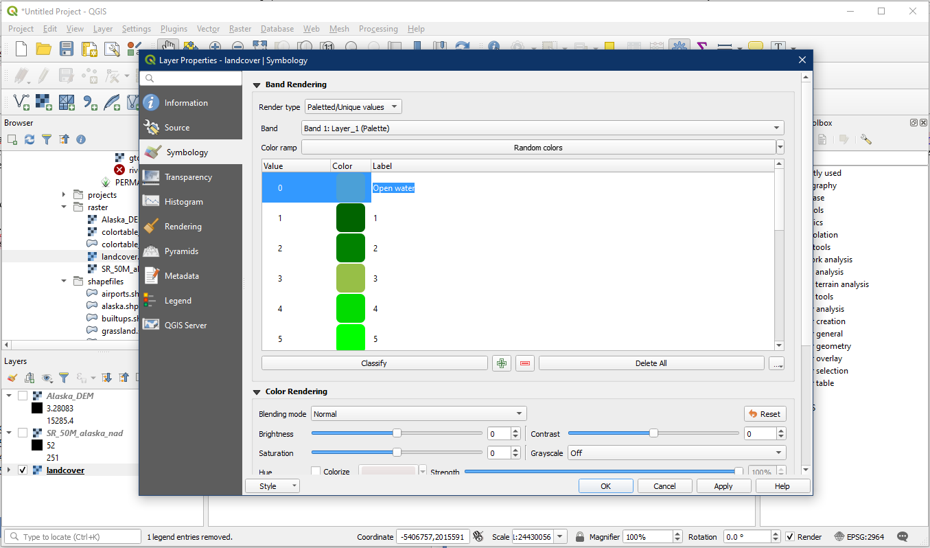
Turn off all layers except the landcover layer properties and look at the Symbology section. You will see 14 values of landcover where the labels are displayed as the numbers 0 to 13. These labels are not very useful, so using the classification table below, rename the Label column in the Symbology by double clicking the numbers in the Label column and typing in the land cover name. For example replace “0” with Open water.

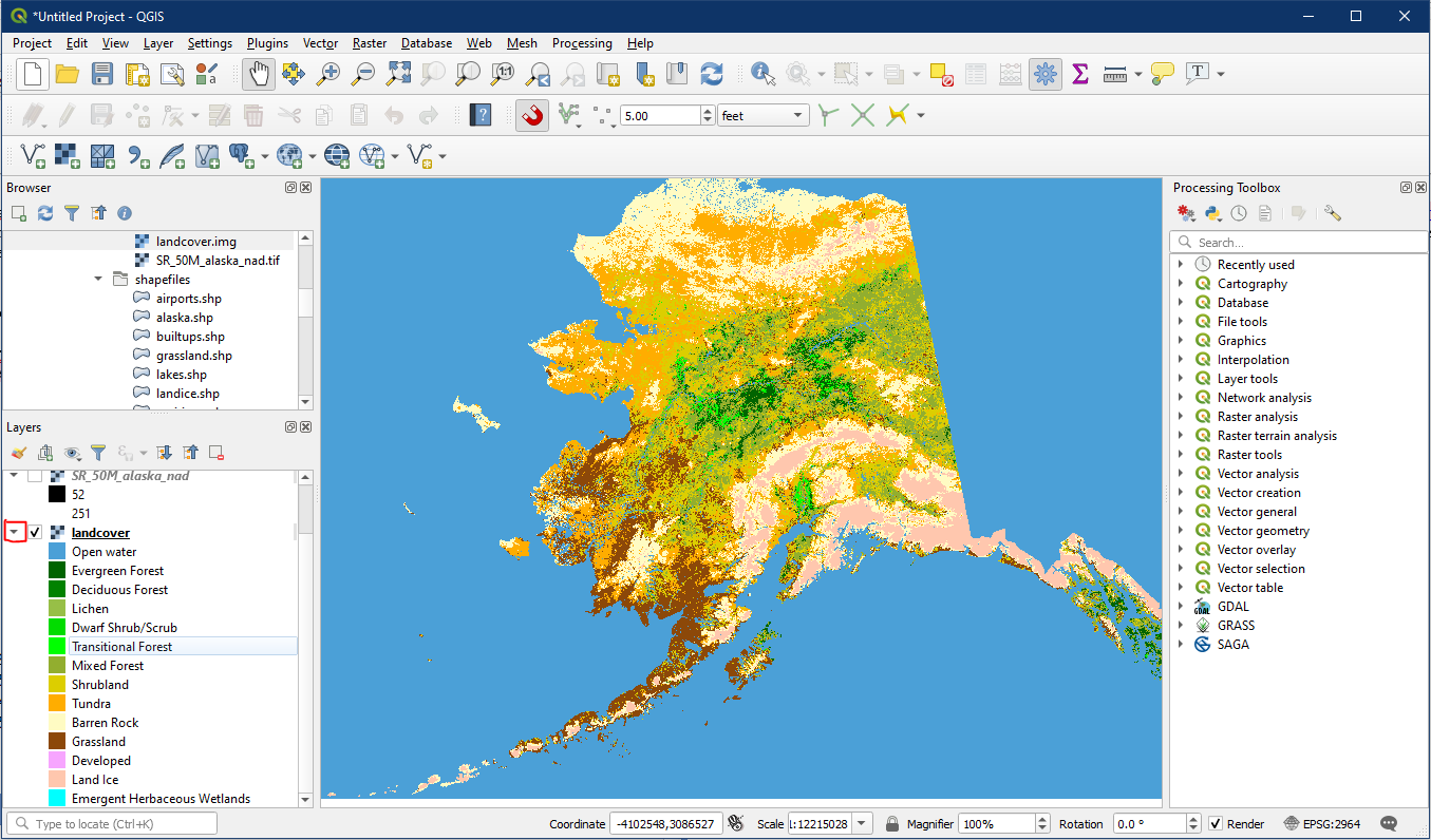
When that is complete, click the triangle beside the landcover layer in the Layer Panel and it will now display the full land cover types with the proper names that we have entered.

Quantitative Raster Data

This method of classifying data is often used in raster data format because the cells only have a single attribute.

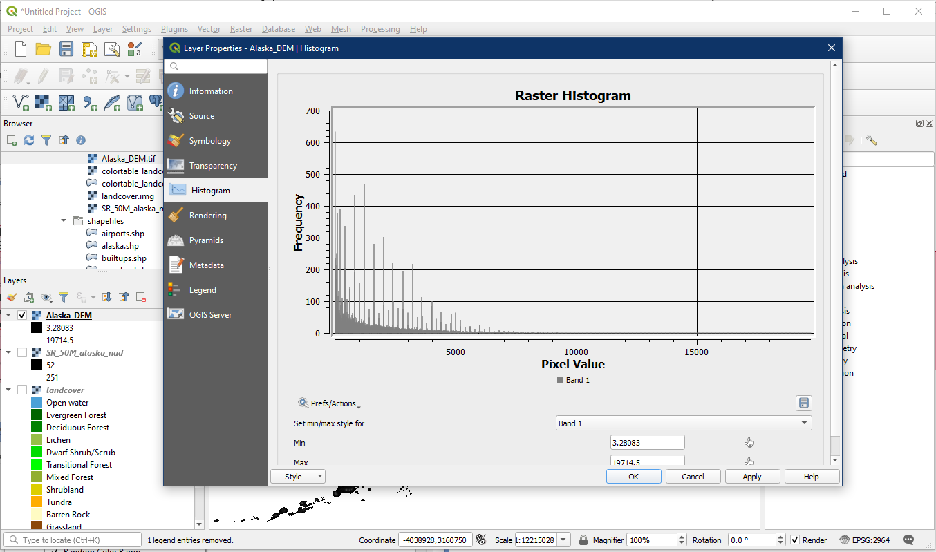
Turn off all layers except the Alaska_DEM layer, which illustrates the elevation. Go to the layer properties and open the Histogram section. You may need to click the “Compute Histogram” button if there is nothing in the histogram. This will produce a histogram which illustrates the distribution of elevations in the area. Notice the majority of the pixels are low in elevation (high frequency of low elevation pixels). You will see the minimum (Min) elevation and the maximum (Max) elevation listed under the histogram.

Go to the Alaska_DEM Symbology section. By default the Render type should be Singleband gray.

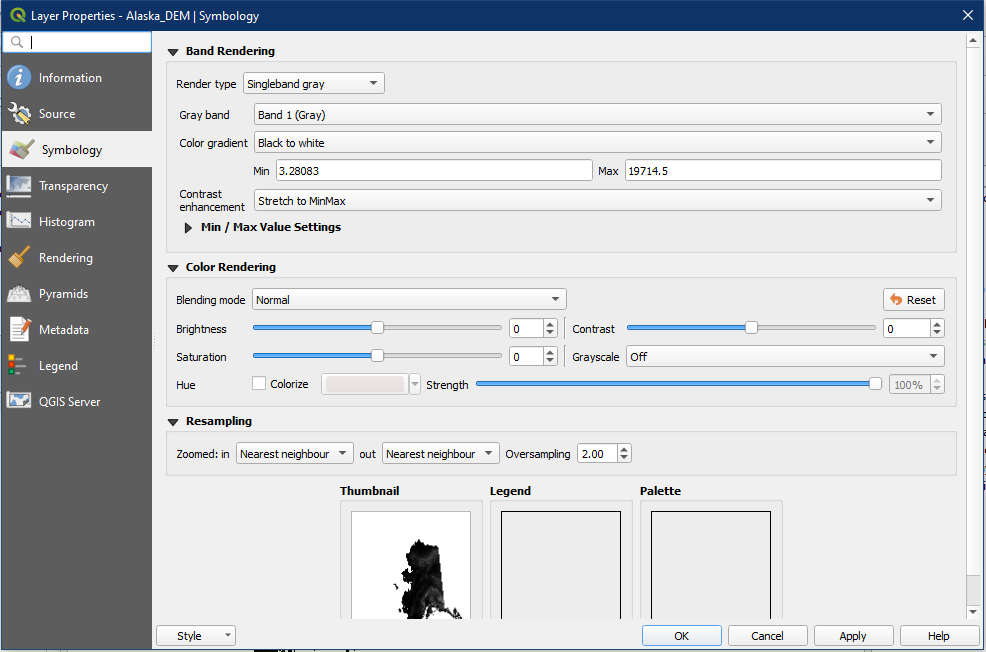
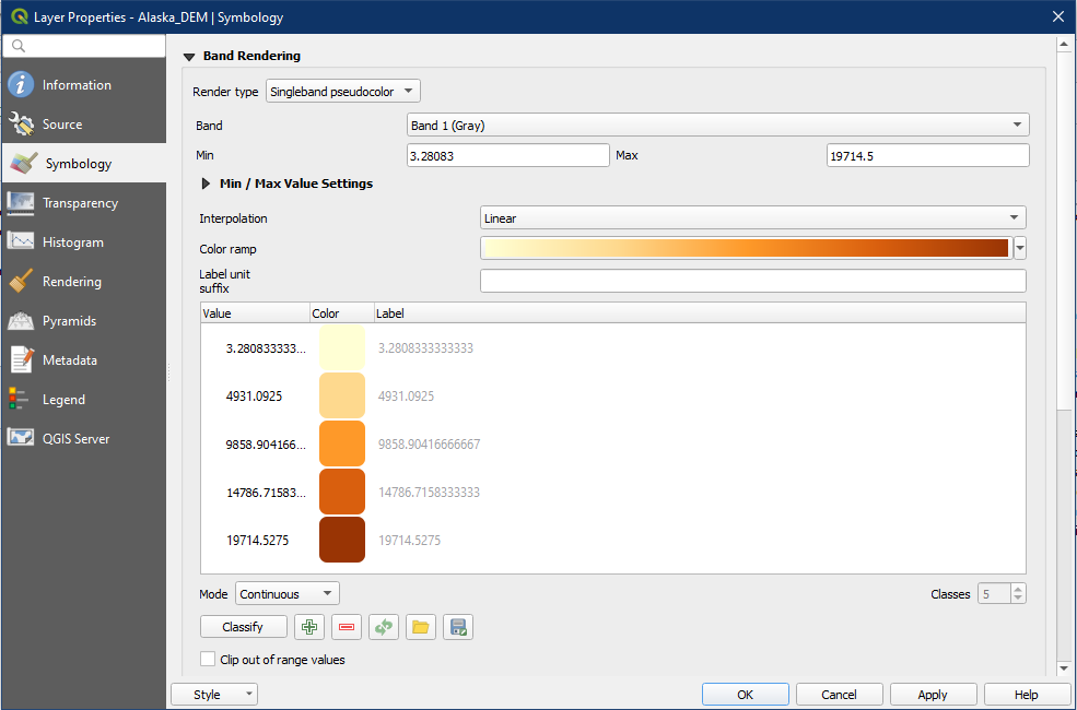
We will be changing from Singleband gray to a graduated elevation colour ramp. Change the Render type to Singleband pseudocolour.

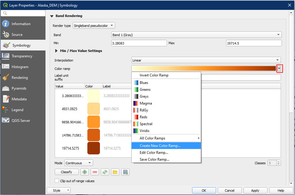
In general DEM most often employ a similar colour ramp which is not one of the default options, but exists in the built-in catalogue. To access it, click the arrow beside the Colour ramp, and select Create New Colour Ramp.

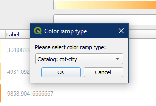
In the Colour ramp type window popup, choose Catalog: cpt-city. Click OK.

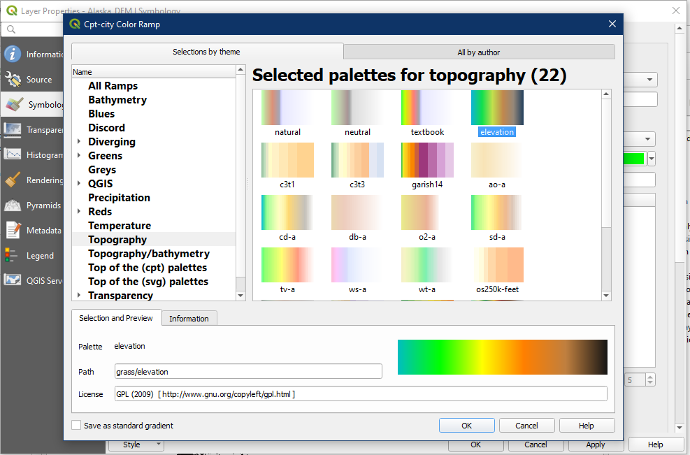
The Cpt-city Colour Ramp window will open. There are many great colour ramps found here that you can browse through and use. For now, select the Topography category and pick the elevation colour ramp. Click OK.

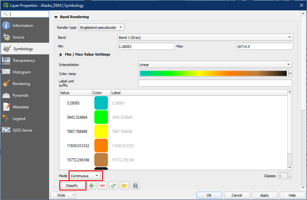
The new colour ramp should now be reflected. For the Mode, choose Continuous, which gives us an even distribution of the colours. Make sure to always click the Classify button to update the changes, since QGIS usualy does not do it by default. Click OK.

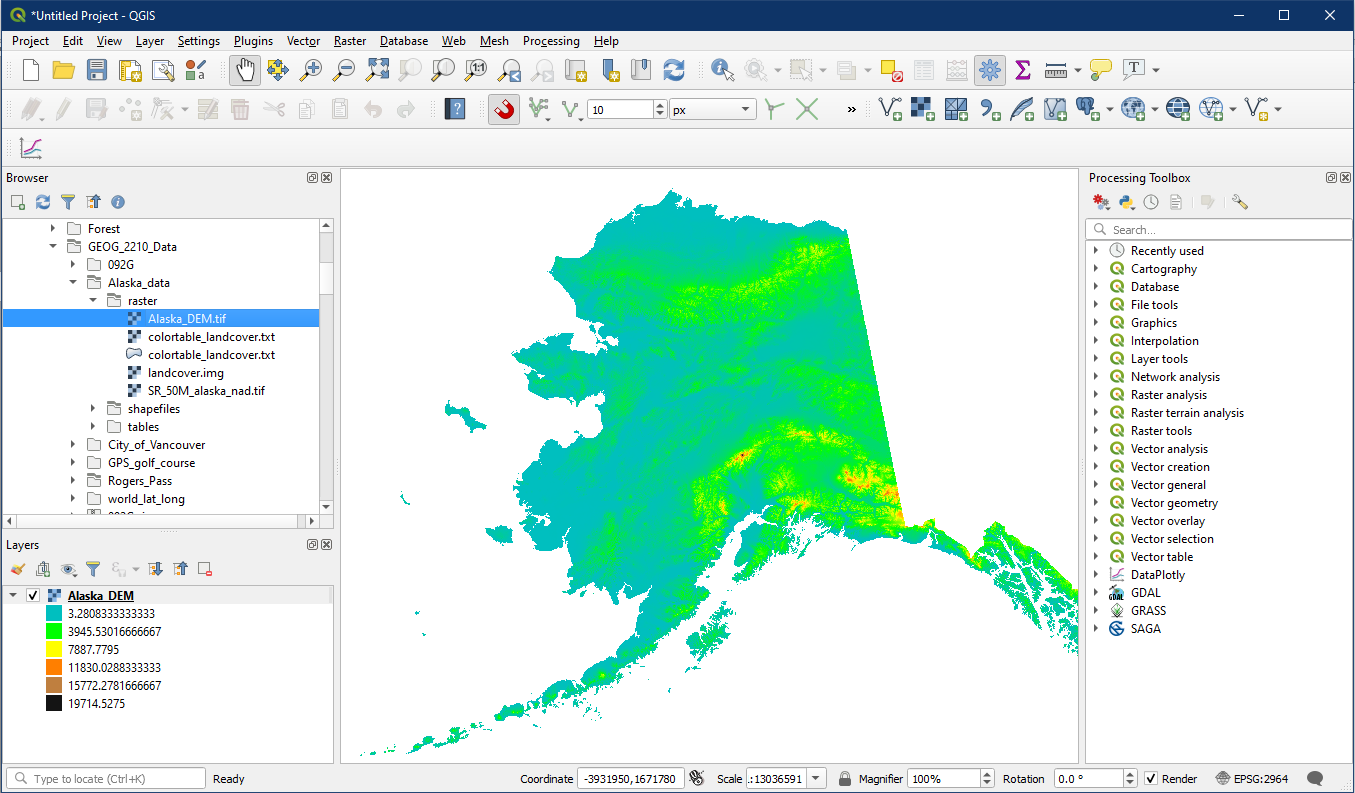
The Alaska_DEM layer should now be displayed using the elevation colour ramp. This colour ramp provides a better indicator of elevation change to the map reader and improves the effective conveyance of elevation differences.

Now turn on all three raster layers and place them in the following order:

1. SR_50M_alaska_nad
2. Alaska_DEM
3. landcover

The Alaska_DEM layer is a Digital elevation model with a 30 metre pixel size, and SR_50M_alaska_nad is a hillshade. If you are zoomed in you can really notice the difference between the pixel sizes of these two raster layers.

Go to the layer properties for SR_50M_alaska_nad. Go to the Transparency section, and under Global Opacity change it to 60% (we did this in tutorial 5). Pan out and take a look. The DEM is improved by the hillshade and the colour ramp. We often pair raster files in this manner to improve the appearance of elevation difference. Turn on the landcover layer to display oceans in the background. Save your project as Tutorial_10.