Overview

Historically, geospatial information was stored on hard copy maps. To create digital databases of that geospatial information it was necessary to transfer the information from those maps to a database. This was accomplished by using devices (digitizing tablets or tables) to “trace” the points, lines and areas on the maps and convert them to digital files. This process was referred to as digitizing. Presently, vast amounts of geospatial data are available as digital files and the need to digitize information from hard copy maps has been greatly reduced.

The wide availability of georeferenced digital imagery (orthophotos, satellite imagery etc.) has changed the nature of digitizing significantly. A common GIS task is the creation of a vector layer by digitizing the features shown on a digital image. This is called heads-up digitizing.

QGIS provides some basic digitizing capability through its digitizing module. This tutorial introduces the use of that module. More sophisticated digitizing programs are available, including the commercial application CartaLinx, which is available on the Langara network.

Digitizing Map Data

Digitizing is one of the most common tasks that a GIS Specialist has to do. Often a large amount of GIS time is spent in digitizing raster data to create vector layers that you use in your analysis. QGIS has powerful on-screen digitizing and editing capabilities that we will explore in this tutorial. For additional resources and if you find you have made a mistake and need to remedy the situation or want more advanced knowledge beyond this tutorial, visit the QGIS reference manual this is very helpful

Overview of the task

We will use a raster topographic map and create several vector layers representing features around Langara College.

Activity 1: Initial Setup

Before we begin the process of digitizing we need to open the QGIS program. In the Browser portal navigate to the City_of_Vancouver folder in your data folder.

Our desire is to digitize in a specific projection. I suggest the following steps to avoid confusions about projections. We will learn more about projections in lecture and in the next lab.

Open Project > Properties > CRS section

Alternatively, click the EPSG button on the bottom right corner.

Either way, in the Project Properties CRS section, search for “26910” (A). Then click on the filtered result below (B), with a Coordinate Reference System of NAD83/UTM zone 10N and an Authority ID of EPSG:26910. Once it is selected and highlighted in blue, click OK.

The bottom of your QGIS window should now show EPSG:26910.

You are searching for an ESPG code. ESPG is explained here (read this because it is interesting and I like to test on interesting things). Here is a link to a library of codes. Go to this website and enter “26910” into the codes area. Then view the information about the code. This information will prove valuable later in life. I am also a fan of this Spatial Reference List . These reference sites are great for picking up the extents or boundaries of different projections, something we will be doing in this course.

You have now set your projects Coordinate Reference System to ESPG Code 26910, which is a NAD 83 datum and a UTM zone 10. Understanding what this means is critical, so I turned to GOOGLE and found this. NAD 83 is a datum or geometric datum (reference points that provide accurate locations corrected for distortion, remember Earth is not a perfect sphere and is distorted).

Universal Transverse Mercator (UTM) is a projected coordinate system that provides an organized reference system for locations (similar to Latitude and Longitude, but metric and different). Since Vancouver is in Zone 10 we are going to use UTM Zone 10

Activity 2: Digitizing Points

Navigate to the Orthophotos_2015 within the City of Vancouver folder and open the raster layer Langara_Orthophoto_2015 by dragging it into the map area.

Langara_Orthophoto_2015 is the base layer that we will use to create vector layer by digitizing. In essence the raster layer guides your digitizing process.

More on Orthophotos in BC and this set of 2015 orthophotos. If you read about the orthophoto you would discover it has a 6.5 cm pixel size. Is this true? How would you know? Check the Layer Properties.

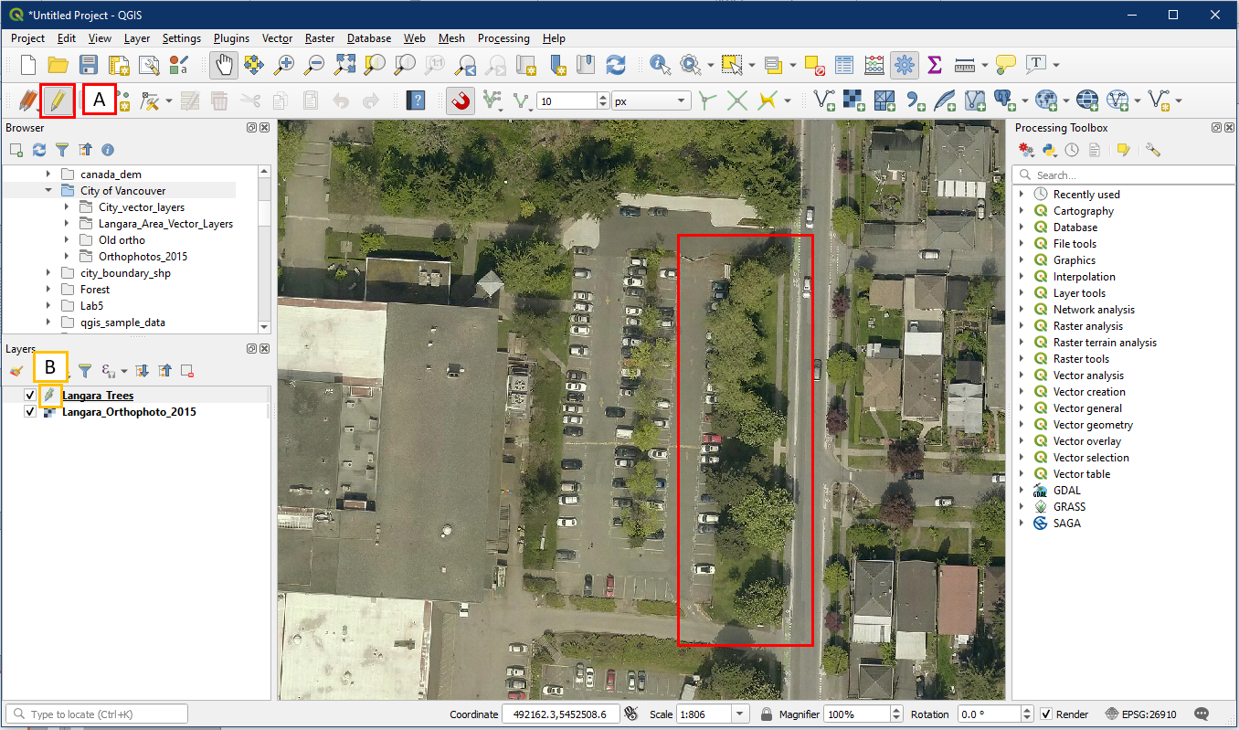
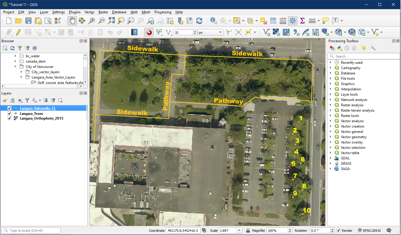
Your QGIS display will look similar to this. In the main QGIS window, use the navigational buttons (A) and your scroll wheel or Page Up/Down keys to locate Langara College. This is the location we will be digitizing. Imagine that you want to create a point vector layer that you will use to show the location of trees on a portion of the Langara Campus. This example will illustrate how to digitize the position of the trees within the highlighted area (B). Tip: You can hold the CTRL key while scrolling the mouse wheel for better zoom control.

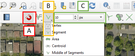
Before we start, we need to set snapping options. Ensure that the Snapping Toolbar is turned on (recall tutorial 3), it should look like this.

We will need to configure the following options to ensure snapping works well:

1. Ensure the Enable Snapping button (magnet) is turned on
2. Choose Vertex and Segment
3. Set 10 px (pixels)

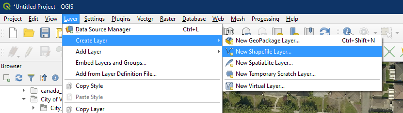
Now to begin Digitizing. In the menu click Layer > Create layer > New Shapefile Layer

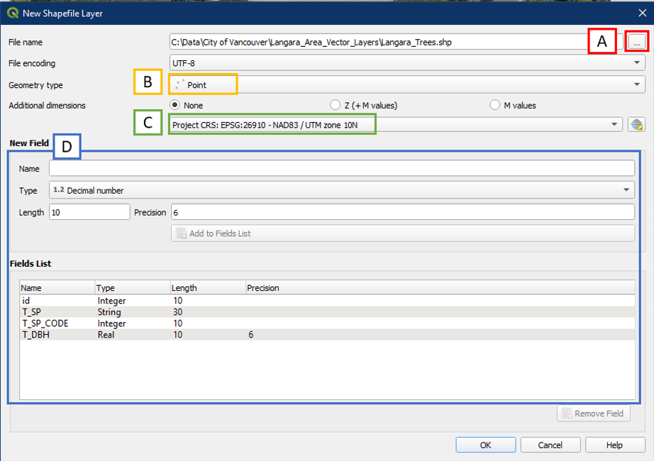
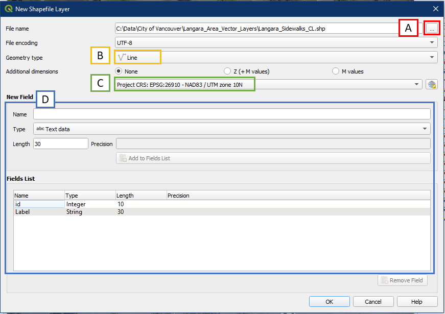
In the New Shapefile Layer window, fill in the following:

1. File Nameof Langara_Trees using the browse button “…” it in the Langara_Area_Vector_Layers folder. Remember, don’t type into the File name box!
2. Geometry Type = Point
3. Choose ESPG:26910 (this should be the same EPSG code as the one found in the lower right corner of our QGIS window, aka our project CRS)
4. In order to properly provide and organize the attributes we need to create fields for our attribute table. Using the New field box, we will add the attributes

• *Note that the field type has a different naming convention in the added list. Whole number = Integer. Decimal number = Real or Double. Text data = String.
• If you make a mistake, click the Remove Field button to delete that field and add it again

You can always add new fields or rename existing fields at a future time. To do so, open the layer’s attribute table.

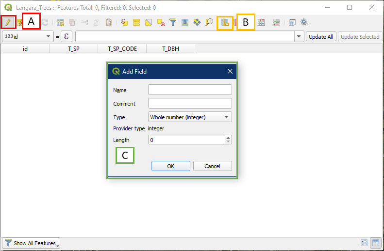
1. Click the Toggle Editing button to turn on editing
2. Then select the New Field button which will open the Add Field window (C).
3. Fill in the Add Field box like we did when creating the Shapefile. When done, click the Toggle Editing button (A) again to turn off editing.

Now we are ready to start digitizing the trees and we can begin by clicking the Toggle Editing button (A) to turn on editing. We want to digitize points showing the position of the trees in the highlighted areas. Start by zooming into the highlighted portion of the image so you can clearly see this strip. Note that in the Layers panel, the Langara_Trees layer now has a yellow pencil over the symbol (B), this means the layer is in edit mode.

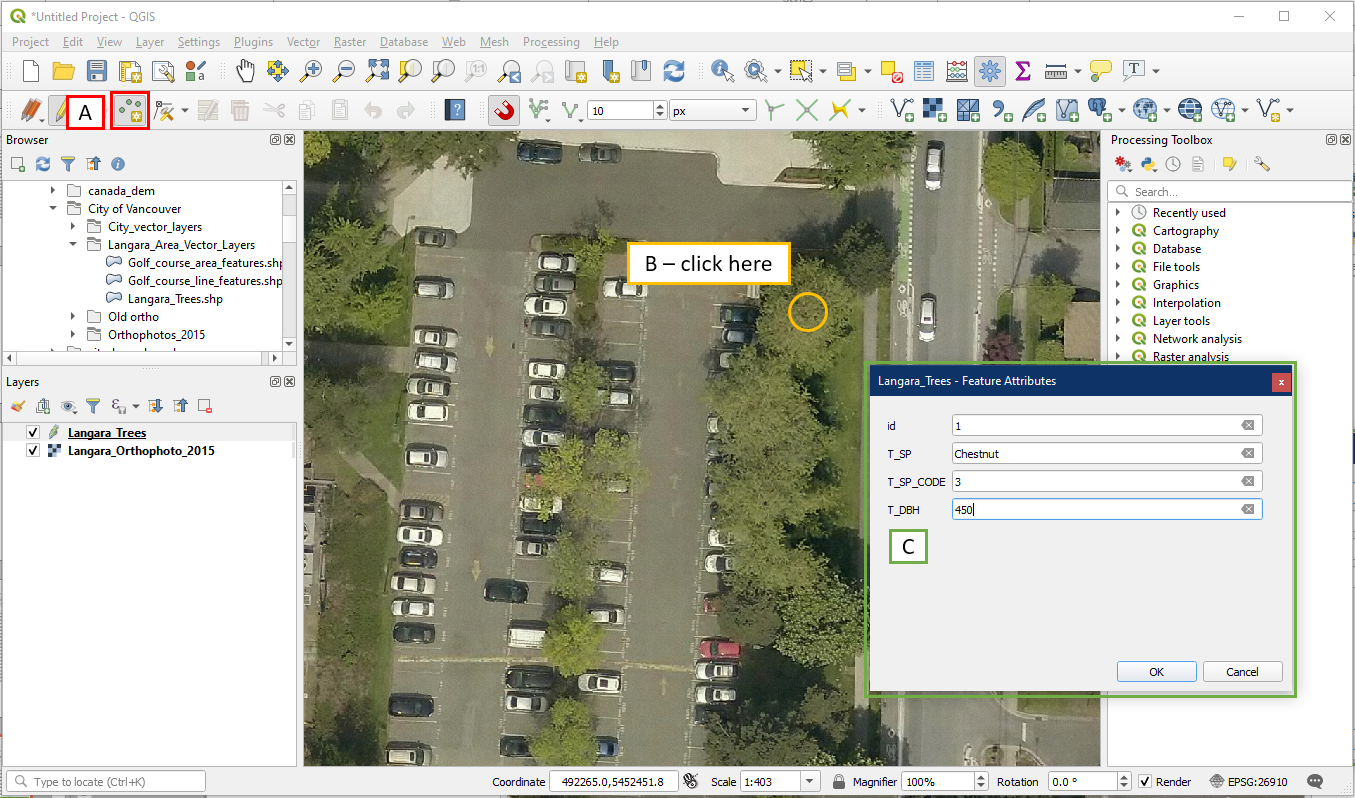
Select the Add Point Feature button (A). Position the cursor over a tree and left click the centre of a tree as shown below (B). The Feature Attributes window (C) should pop up. For practice purposes, let’s imagine that we have surveyed this tree and it is a Chestnut, has a species code of 3, and a diameter of 450 mm. Enter these information in the appropriate boxes. For id, give it a value of 1 since this is our first record. Click OK when you are done.

You simply repeat the process to digitize more point features. Try digitizing all the trees on this grass patch. Remember to give each new point a new id, so your second point should be id = 2, and third point would be id = 3 etc. But you can leave the other fields blank for now.

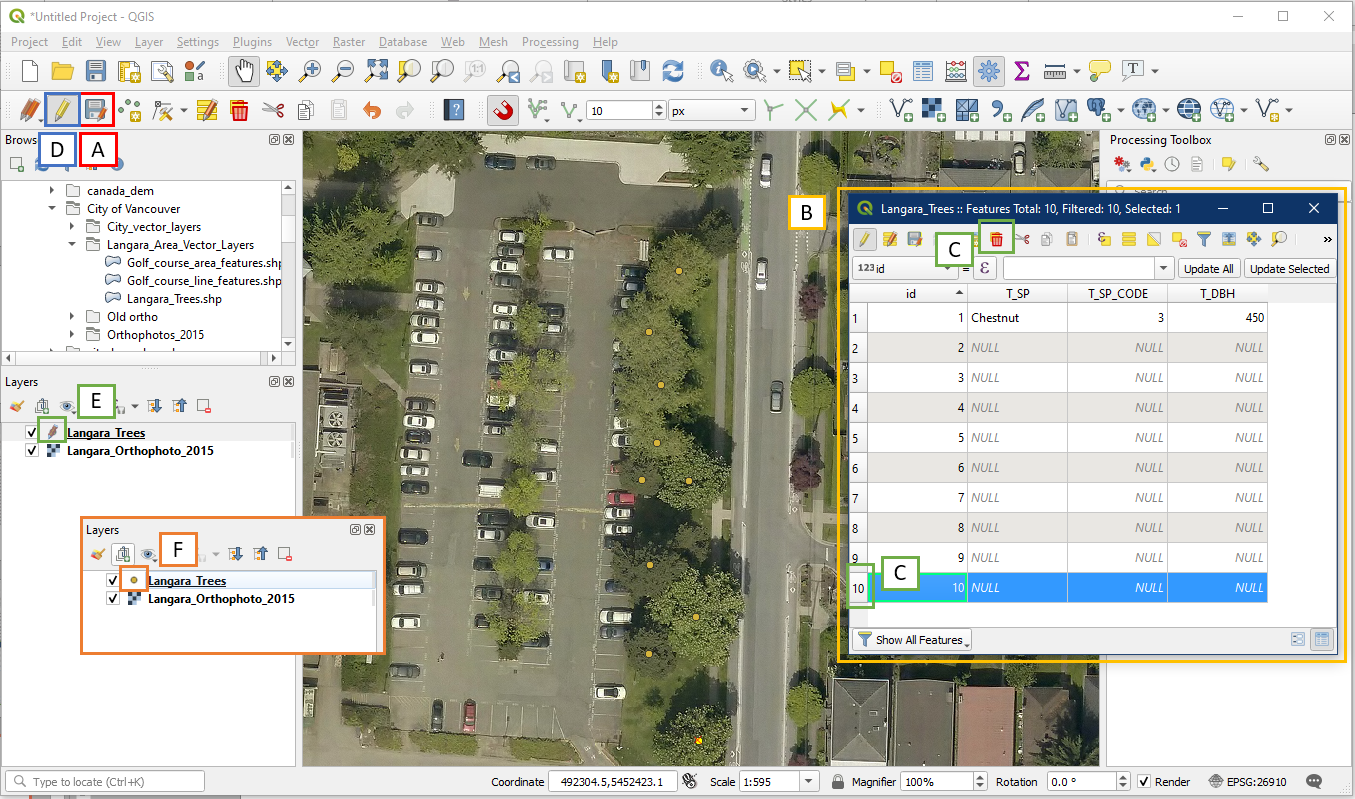
It is a good idea to periodically save your work using the Save Layer Edits button (A). You can view your progress in tabular form by right clicking on the Langara_Trees layer > Open Attribute Table. In the Attribute Table (B) you can update the attribute information by typing into the field boxes. You can also delete records by highlighting the record using the number on the left and choosing Delete Selected Feature (C). Once you are done, click the Toggle Editing button (D) to turn off editing. If there are any unsaved edits, the yellow pencil beside your Langara_Trees layer will be red (E). Once you turn editing off, the pencil symbol should disappear (F). It is a good habit to always check your Layers panel for unsaved edits (red pencil). It is also a good habit to keep the editor off when not in use (no more pencil shown for any layer).

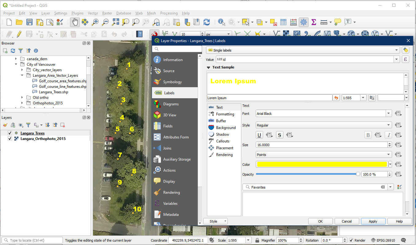
Now that you have created multiple points with unique Tree Species Identification codes you may want to display the codes. Right click the layer in the Layers Panel, Open the Properties > Labels and choose Single Labels for this layer, and under Value the id field. You can also choose colour and size etc.

Now would be a good time to save your project. Save it as Tutorial_11.

Probably the biggest challenge in digitizing points representing the position of the trees from this orthophoto is the fact that when viewed from above the trees are not point features. The tree canopies obscure the actual position of the tree stems. To represent the tree using a point symbol requires that you make an estimation of the position of the tree.

An alternative would be to digitize areas to represent the space occupied by the tree canopies, but the resultant map might not be too useful to the user on the ground attempting to identify individual trees.

Remember the features on a map are symbolic representations (using points, lines and areas) that represent real world features. The scale and the purpose of the map will determine how those symbols are used.

Activity 3: Digitizing Lines

Before you begin digitizing linear features it is important to learn some digitizing terminology.

A line (also referred to as an arc) consists of straight segments that connect vertices. A single vertices is a vertex.
Lines start and stop at nodes. The intersection of two or more lines is also at a node. When you were digitizing trees in the previous section you were digitizing points, not nodes. The following image shows examples of the different features in the Digitize view.

In QGIS, open your Tutorial_11 project. It should contain the Langara orthophoto and the Langara_Trees point layer. We will be digitizing in the area just northwest of our Langara_Trees layer as shown below.

Again, create a new shapefile vector layer. This time we are going to create a line vector layer named Langara_Sidewalks_CL. CL stands for centreline. This will be similar to how we created the Langara_Trees point layer.

1. Remember to use the “…” button to save your layer name and folder location.
2. For Geometry type choose Line. In newer versions of QGIS it’s called LineString.
3. Choose EPSG 26910 to match our project
4. Add one extra field called “Label” that is Text data (String) and a Length of 30.

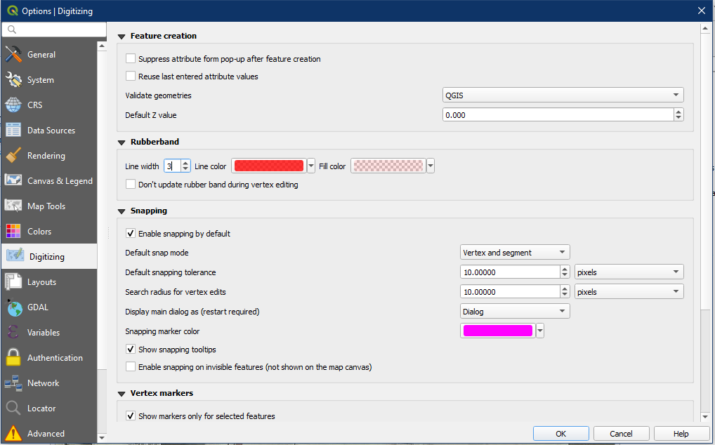
To make editing lines easier to see, we will first go into Settings > Options.

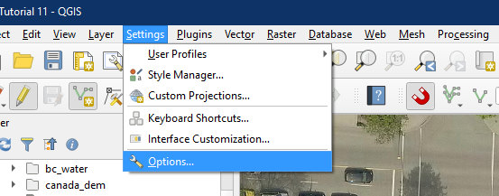
Go to the Digitizing section. Under Rubberband, choose a Line width of 3. This will thicken the edit line, making it easier to see. Click OK.

Generally all the digitizing tools work in a similar fashion.

1. Left click on an icon to select the tool.
2. Left click to perform the tool function, or select the features that the function will be performed on.
3. Right click to complete the function.
4. The tool remains selected until another tool or icon in the menu bar is selected.

Here are the steps to digitizing our first line:

1. Make sure our Snapping Toolbar options are set as described in the Digitizing Points section.
2. With Langara_Sidewalks_CL selected, toggle on editing
3. Select the Add Line Feature (note that this button changes to Add Point/Line/Polygon based on the layer type)
4. Left click a starting point. Left click again at each junction to create turns.
5. When the line is finished, right click anywhere to complete the line
6. The Feature Attributes window should pop up. Enter id = 1, and Label = Pathway. Click OK
7. For best practice, make sure to save

As you are digitizing you can use the Map Navigation buttons, your arrow keys, or holding down the middle mouse button to change the view.

A useful tool to help you with digitizing is the Vertex Tool. Click the Vertex Tool button (A). Once the vertex tool is activated, hover over any feature to show the vertices. Click on any vertex to select it (B). The vertex will change the color once it is selected, you can drag your mouse to move the vertex to a different location (C). This is useful when you want to make adjustments after the feature is created. You can also delete a selected vertex by selecting it and clicking the Delete key (Option+Delete on a mac).

For our second line, select the Add Line Feature button again and draw a line from A to B. Since we set a snapping tolerance of 10 pixels to vertex and segments in the Snapping toolbar, the second line will snap to the existing point at B once you’re the cursor is close enough. Right click when your line is complete, and in the Feature Attributes window (C) enter id = 2, and Label = Sidewalk.

Try to digitize a few more sidewalks and pathways to become familiar with creating and editing lines. You should end up with something like this. Remember to always save (A) if there are unsaved edits (red pencil shown beside the layer name). Then toggle edit off (B). Ensure no pencil symbols remain beside the layer name (C).

Imagine we want to find out how long the sidewalks and pathways are on campus. We can do this by creating a new field and using it to calculate length.

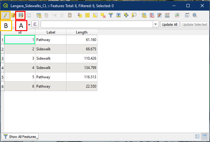
Recall earlier that you can create and modify fields after the Shapefile has been created. To do so first open up the Langara_Sidewalks_CL attribute table.

1. Click the Toggle Editing button to turn on editing
2. Then select the New Field button which will open the Add Field window (C).
3. Fill in the Add Field box with the following details. When done, click the Toggle Editing button (A) again to turn off editing.

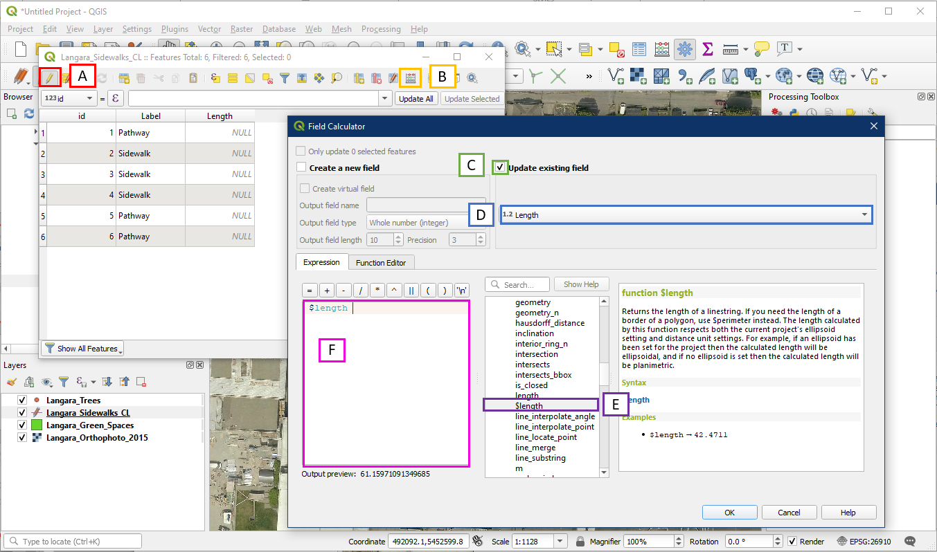
Now we can calculate this field. To do so:

1. Turn on Toggle Editing Mode again
2. Click the Open Field Calculator button
3. Check the box for Update Existing Field
4. Choose the new field, Length
5. In the function box find $length under the Geometry section. Double click on $length
6. $length should show up in the Expression box. It will also display an example output preview. Click OK

Your Length field should now be populated with the length. We know this is in metres squared because the units for this layer are in metres (check in layer properties). Make sure to save your edits (A) and turn off editing (B) when done.

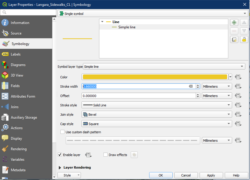
The default line is thin and hard to see. You can increase the line thickness (Stroke width) under the layer properties under Symbology.

Also label the layer using the Label field. Give it a larger font and brighter colour.

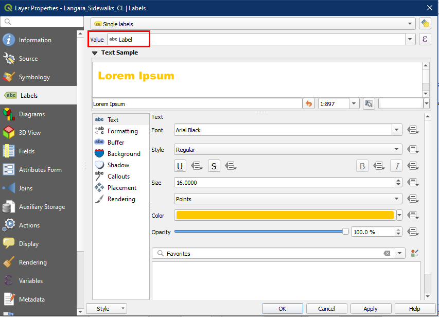
Your lines should now be labelled and are easier to see.

Save your project before advancing onto the next activity

Activity 4: Digitizing Polygons or Areas

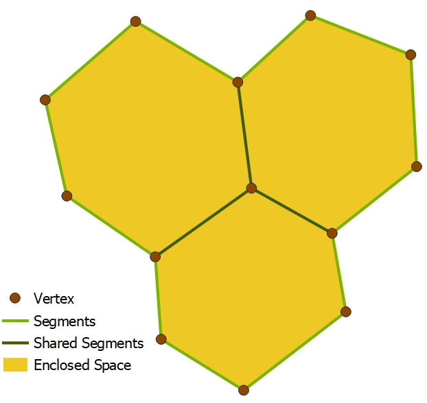
Digitizing area features is a little bit more complex than digitizing points and lines because an area feature has two components

• An enclosed space, defined by a boundary made up of segments and vertices.
• A centroid that indicates this enclosed space is an area.

Furthermore, adjacent areas share boundaries.

Open QGIS and continue your Tutorial_11 project, you will want to open the Langara_green_spaces layer found in the Langara_Area_Vector_Layer folder. As you will find out in the class projects later on (and possibly in your future GIS work), much editing work are done on existing datasets. You will notice that some of the green spaces on the Langara Campus are covered with polygons. Turn off the line and point layers if they are distracting.

Now we will continue to digitize in this Langara_green_spaces layer. Alternatively you can create your own layer for practice. Zoom into the highlighted area.

The steps to adding a new feature is very similar to creating lines, except that the lines created will enclose an area.

1. Make sure our Snapping Toolbar options are set as described in the Digitizing Points section.
2. With Langara_Green_Spaces selected, toggle on editing
3. Select the Add Polygon Feature (note that this button changes to Add Point/Line/Polygon based on the layer types)
4. Left click any corner to start, and proceed to add each corner in either clockwise or counter clockwise order around the planting bed
5. When all corners of the area are finished, right click anywhere to complete the line
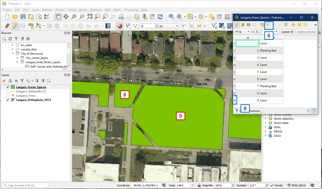
6. The Feature Attributes window should pop up. Enter id = 7, and Label = Planting Bed. Click OK
7. For best practice, make sure to save

Once that is done, try digitizing these two polygons (id 8 and 9). These will be Lawns. Recall that if you make a mistake recall that you can select the number beside the row and click the Delete Selected Features button (B) to remove it.

Imagine that we want to find out the area of green spaces on the Langara campus. We can do this by creating a new field and using it to calculate area.

This is the same method as calculating length for lines. To do so first open up the Langara_Green_Spaces attribute table.

1. Click the Toggle Editing button to turn on editing
2. Then select the New Field button which will open the Add Field window (C).
3. Fill in the Add Field box with the following details. When done, click the Toggle Editing button (A) again to turn off editing.

Now we can calculate this field. To do so:

1. Turn on Toggle Editing Mode again
2. Click the Open Field Calculator button
3. Check the box for Update Existing Field
4. Choose the new field, Area
5. In the function box find $area under the Geometry section. Double click on $area
6. $area should show up in the Expression box. It will also display an example output preview. Click OK

Your Area field should now be populated with the area. We know this is in metre squared because the units for this layer are in metres under layer properties. Make sure to save your edits (A) and turn off editing (B) when done.

You have now succeeded in digitizing points, lines, and polygons. You have the ability to navigate attribute tables and edit. These are useful skills to have for this class as well as being a necessity in the GIS world.

Please save your QGIS project.

Well done!!!