Please read sections 10.1 to 10.6 from the QGIS page on Buffers: Vector Spatial Analysis Buffers

In the following we will conduct a buffering exercise to conduct spatial analysis to answer the question: What is the average number of children between the ages of 0-14 years of age that live in a neighbourhood that overlaps a 500 metres buffer around the Carnegie, Strathcona, Britannia, and Hastings libraries?

Before you begin the process of answering the question, first ask yourself what data is needed?

• the location of the four libraries
• the average number of children residing within 500 metres of the libraries
• a 500 metre buffer surrounding each library

Activity 1: Selecting Areas of Interest and Creating a Buffer

To begin open a new QGIS project. Add the following layers:

• Census_Neighbourhood_2016_age from the Census folder
• libraries from the Cultural folder

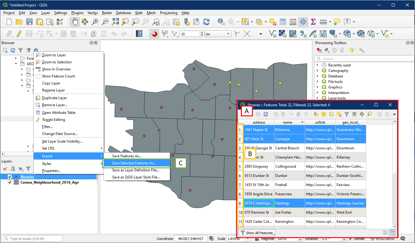
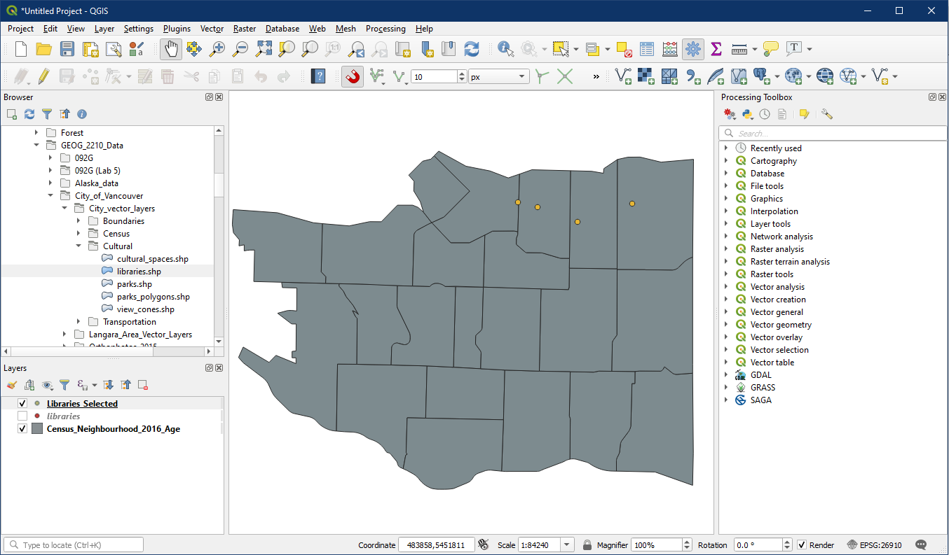
Open the attribute table (A) for the libraries layer and select the four libraries mentioned above (Carnegie, Strathcona, Britannia, and Hastings). Use CTRL while click the numbers beside the records (B) to highlight multiple records at once, notice that they will also be highlighted as yellow points on the map. Once these four libraries are selected, right click the layer > Export > Save Features As, and save it as a new point layer.

In the Save Vector Layer as window, set the following:

1. Choose ESRI Shapefile as the format
2. Click the “…” button to specify the folder location and file name

The new layer will contain only the libraries we want to use.

To create buffers around these libraries, use the Buffer tool:

1. Vector > Geoprocessing Tools > Buffer
2. Processing Toolbox > Vector geometry > Buffer
3. Search box

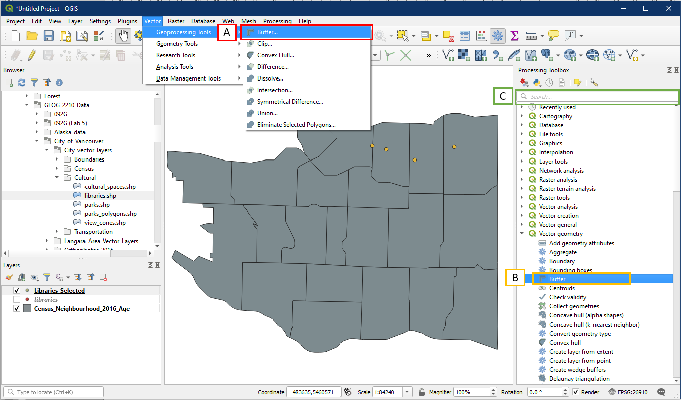
In the Buffer dialog window, choose the following:

1. For Input layer choose the new selected libraries layer
2. Choose a distance of 500 metres
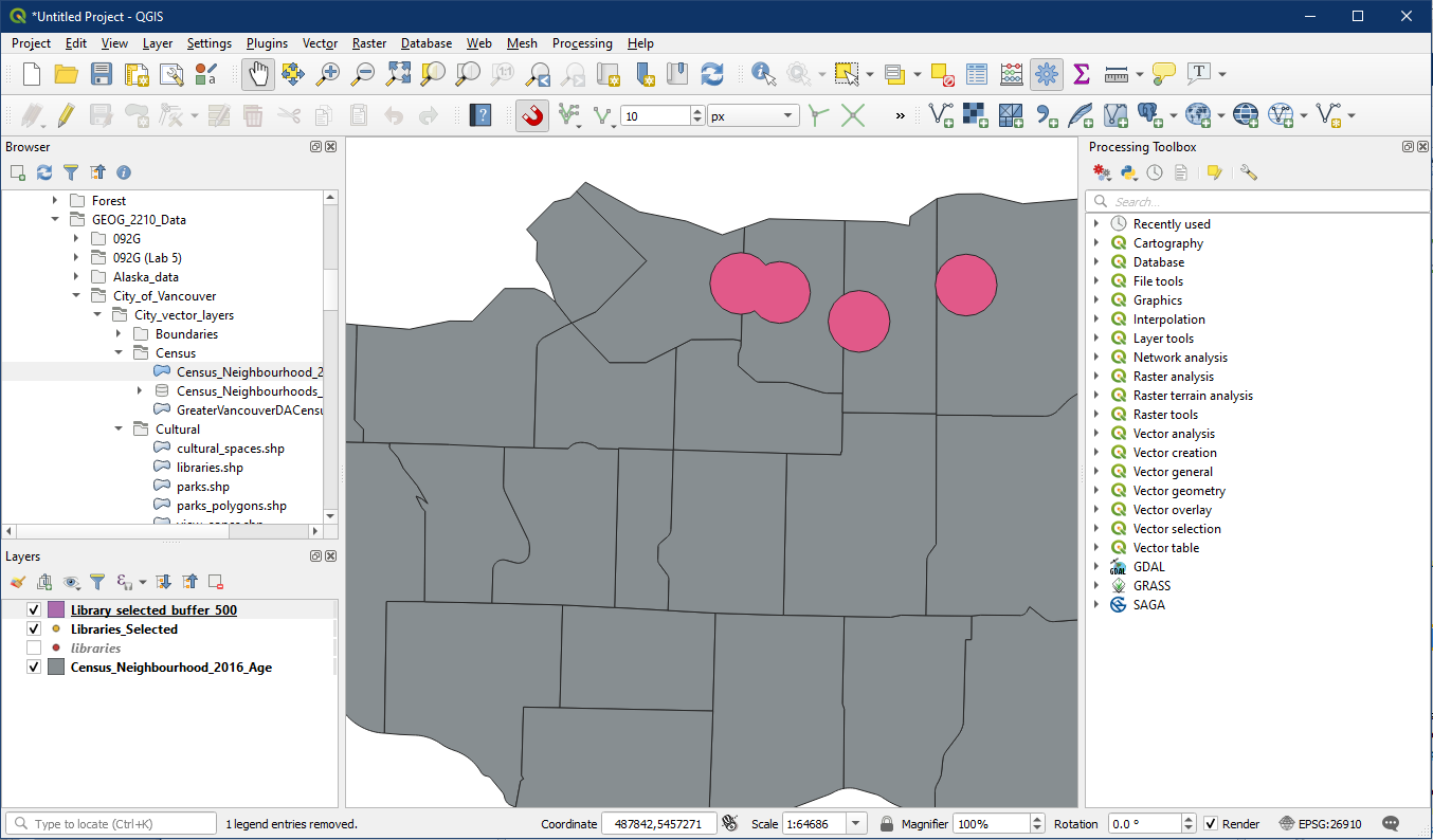
3. Check Dissolve Result – this will prevent buffer boundaries from overlapping, and instead will only create outer boundaries for overlapping buffers
4. Click the “…” to Save to File, specify the folder location and file name of the buffer layer

It will look something like this:

To see which neighbourhood blocks coincide with these buffered areas, go to Processing Toolbox > Vector selection > Extract by location (A). Alternatively search for it in the search box (B).

In the Extract by Location window, select the following.

1. Extract features from the Census_Neighbourhood_2016_Age layer
2. Check intersect option
3. By comparing to the features from the buffered library layer
4. Click the “…” button to Save to File, select a folder location and file name for the extracted layer

The new layer will contain all the neighbourhoods that touch the buffers. This is a similar process to the Clip tool we used in tutorial 20, but the Extract by location preserves the entire neighbourhood boundaries, whereas the Clip tool would have clipped the neighbourhood boundaries to match the buffers.

If we are making a map we may want to symbolize the selected neighbourhoods to see the number of children within each. Go to the layer properties Symbology section of our new extracted layer and select the following:

1. Choose Graduated mode
2. For Value choose the field “0 to 14”
3. Choose a colour ramp of your choice
4. Pick Equal Count (Quantile) mode – this mode is great at showing an even distribution of colours
5. Click Classify – always click this button after making changes to symbology

If we make a map now we will be able to tell that certain neighbourhoods contain more children.

Activity 2: Vector Statistics

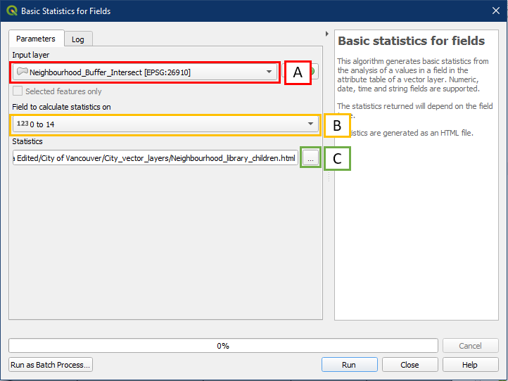
To produce vector statistics, pick one of the following options to open the Basic Statistics for Fields tool:

1. Vector Menu > Analysis Tools > Basic Statistics for Fields
2. Processing Toolbox > Vector Analysis > Basic Statistics for Fields
3. Search box

In the dialog window, choose the following:

1. For Input layer select your intersected neighbourhood layer
2. For Field to calculate statistics on, choose the “0 to 14” field
3. Click the “…” button to Save to File, specify a folder location and file name for the output

The tool will produce an HTML output that can be opened in any browser. It will contain a list of statistics. The following are particularly useful for us.

1. Count – the total number of records within the layer. In this case 4 neighbourhoods were analysed
2. Sum – the total of all the values within the “0 to 14” field for all records. In this case the total number of children within the selected neighbourhoods is 12870
3. Mean value – the average value of the “0 to 14” field across all records. In this case the average number of children in the selected neighbourhoods is 3217

Great work! Save your project as Tutorial 21.